SQL to Python for Data Analysis: The Practical Translation Guide

Every SQL pattern an analyst uses in a normal week — SELECT, WHERE, GROUP BY, JOIN, window functions, CTEs, CASE, pivots — translated to pandas, with polars and DuckDB alternatives where they read better. Real code, real gotchas, ready to lift.

By Rakesh Madala — 10 years in the data field

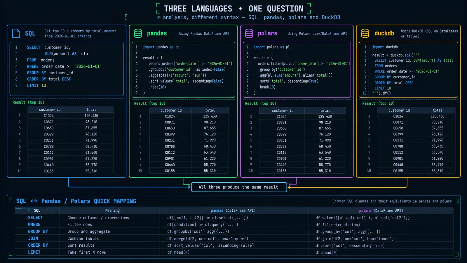
Why a SQL Analyst Learns Python

SQL is what happens inside the warehouse. Python is what happens outside it — when the analysis needs a distribution plot, a survival curve, a scikit-learn model, or an ad-hoc joining of a warehouse table to a CSV that lives on somebody’s laptop. Every SQL-fluent analyst eventually needs to do their work in Python for one of these reasons, and the fastest way to get productive is to map the SQL patterns already in muscle memory to their pandas equivalents.

This is that map. Every pattern an analyst uses in a normal week — SELECT, WHERE, GROUP BY, HAVING, every kind of JOIN, window functions, CTEs, CASE expressions, string and date operations, null handling, unions, pivots, and deduplication — translated to pandas, with polars and DuckDB alternatives noted where they read cleaner. Real code, sample data, and the gotchas that trip up SQL users on their first Python analysis.

The default library in this post is pandas because it’s what a new Python analyst will meet first and what almost every code snippet in Stack Overflow assumes. Where polars or DuckDB genuinely reads more like SQL or runs faster, I note the alternative. For strategic library choice, see the Pandas vs. Polars vs. DuckDB post; this post is about muscle-memory translation regardless of which one you land on.

The setup used in every example

Every code snippet in this post assumes two DataFrames loaded and one warehouse-like sample dataset. If you copy the setup below into a notebook, every snippet will run.

import pandas as pd
import numpy as np

# orders: one row per order
orders = pd.DataFrame([
    {'order_id': 1, 'customer_id': 101, 'order_date': '2026-01-05', 'amount': 120.00, 'status': 'paid'},
    {'order_id': 2, 'customer_id': 101, 'order_date': '2026-01-12', 'amount': 85.50,  'status': 'paid'},
    {'order_id': 3, 'customer_id': 102, 'order_date': '2026-01-08', 'amount': 250.00, 'status': 'refunded'},
    {'order_id': 4, 'customer_id': 103, 'order_date': '2026-02-01', 'amount': 60.00,  'status': 'paid'},
    {'order_id': 5, 'customer_id': 104, 'order_date': '2026-02-14', 'amount': 300.00, 'status': 'paid'},
    {'order_id': 6, 'customer_id': 101, 'order_date': '2026-03-02', 'amount': 45.00,  'status': 'paid'},
])
orders['order_date'] = pd.to_datetime(orders['order_date'])

# customers: one row per customer
customers = pd.DataFrame([
    {'customer_id': 101, 'name': 'Aisha',   'region': 'APAC',   'signup': '2025-10-01'},
    {'customer_id': 102, 'name': 'Bruno',   'region': 'EMEA',   'signup': '2025-11-15'},
    {'customer_id': 103, 'name': 'Chen',    'region': 'APAC',   'signup': '2026-01-20'},
    {'customer_id': 104, 'name': 'Diana',   'region': 'AMER',   'signup': '2025-08-11'},
    {'customer_id': 105, 'name': 'Elena',   'region': 'EMEA',   'signup': '2026-01-30'},  # no orders yet
])
customers['signup'] = pd.to_datetime(customers['signup'])

Notice one thing already: dates arrive as strings from most sources and need pd.to_datetime() to become real timestamps. In SQL the type coercion happens at ingest; in Python you handle it yourself, and every date-comparison bug in a notebook comes from forgetting it.

SELECT and WHERE: The First 90% of Every Analysis

The starting SQL query for almost every analysis is a projection (which columns) and a filter (which rows). In pandas, projection is a list of column names and filtering is a boolean expression.

select order_id, customer_id, amount
from orders
where amount > 100 and status = 'paid';

# selection + filter, verbose form
result = orders[(orders['amount'] > 100) & (orders['status'] == 'paid')]
result = result[['order_id', 'customer_id', 'amount']]

# same thing, chained with .query() (reads more like SQL)
result = (
    orders
    .query("amount > 100 and status == 'paid'")
    [['order_id', 'customer_id', 'amount']]
)

Three things worth noting immediately.

1. Parentheses matter in boolean expressions. Python evaluates & and | with different precedence than SQL’s AND/OR, so orders[amount > 100 & status == 'paid'] without parentheses raises an error. Every boolean clause gets its own parentheses.

2. Use &, |, ~, not and, or, not. The word forms work on single booleans, not on element-wise operations over columns. This is the single most common SQL-to-pandas typo.

3. .query() is the SQL-reader’s friend. It accepts SQL-ish expressions, handles operator precedence sensibly, and is fast enough for most analyses. Multi-condition filters read closer to their SQL origins.

Polars uses a lazier, more explicit API:

import polars as pl
orders_pl = pl.from_pandas(orders)

result = (
    orders_pl
    .filter((pl.col('amount') > 100) & (pl.col('status') == 'paid'))
    .select(['order_id', 'customer_id', 'amount'])
)

DuckDB lets you write literal SQL against Python objects:

import duckdb
result = duckdb.sql("""
    select order_id, customer_id, amount
    from orders
    where amount > 100 and status = 'paid'
""").df()

For SQL-native analysts, DuckDB is often the single fastest ramp into Python — keep writing SQL, get a pandas DataFrame back. This post shows pandas as the primary because that’s where the ecosystem lives, but DuckDB is a valid answer to "how do I do this in Python?" for many of these translations.

Additional filter patterns:

# WHERE status IN ('paid', 'shipped')
orders[orders['status'].isin(['paid', 'shipped'])]

# WHERE status NOT IN ('refunded', 'cancelled')
orders[~orders['status'].isin(['refunded', 'cancelled'])]

# WHERE amount BETWEEN 50 AND 200
orders[orders['amount'].between(50, 200)]

# WHERE order_date BETWEEN '2026-01-01' AND '2026-01-31'
orders[orders['order_date'].between('2026-01-01', '2026-01-31')]

# WHERE customer_name LIKE 'A%'
customers[customers['name'].str.startswith('A')]

# WHERE customer_name ILIKE '%chen%' (case-insensitive)
customers[customers['name'].str.contains('chen', case=False, na=False)]

# WHERE amount IS NULL
orders[orders['amount'].isna()]

# WHERE amount IS NOT NULL
orders[orders['amount'].notna()]

The na=False in str.contains() is a subtle one — without it, string operations on columns that contain nulls return NaN for those rows, and boolean indexing with NaN raises TypeError. Passing na=False tells pandas to treat nulls as non-matches.

ORDER BY and LIMIT

Sorting and taking the top-N rows is one method call each in pandas.

select * from orders
order by amount desc, order_date asc
limit 5;

orders.sort_values(
    by=['amount', 'order_date'],
    ascending=[False, True],
).head(5)

Three details that matter.

1. Multi-column sort passes a list. The by= parameter and the ascending= parameter must both be lists of the same length, and ascending defaults to True for every column if you pass a single bool. Forgetting to align them is a common bug when you convert a SQL query with mixed ASC/DESC.

2. head(N) is LIMIT N; tail(N) is the bottom. There’s no OFFSET equivalent by default — use .iloc[offset:offset+N] after sorting.

3. Null handling in sorts. SQL’s default is engine-dependent; pandas puts nulls last by default. Pass na_position='first' to change it.

# LIMIT 10 OFFSET 20 (rows 21-30)
orders.sort_values('amount', ascending=False).iloc[20:30]

# SELECT TOP 3 by group (like ROW_NUMBER() approach)
(orders.sort_values(['customer_id', 'amount'], ascending=[True, False])
       .groupby('customer_id')
       .head(3))

# nlargest / nsmallest — faster than sort + head
orders.nlargest(5, 'amount')
orders.nsmallest(5, 'amount')

nlargest / nsmallest are worth remembering — for a top-N query on a large DataFrame, they avoid a full sort and are dramatically faster than sort_values().head().

GROUP BY, HAVING, and Aggregation

The single most translated pattern from SQL to pandas is the GROUP BY ... aggregate shape. Get the pandas equivalent right and half of an analyst’s daily work translates cleanly.

select
  region,
  count(*) as order_count,
  sum(amount) as total_revenue,
  avg(amount) as avg_order,
  min(order_date) as first_order,
  max(order_date) as last_order
from orders o
join customers c on c.customer_id = o.customer_id
where o.status = 'paid'
group by region
having sum(amount) > 100
order by total_revenue desc;

The pandas translation:

result = (
    orders
    .merge(customers, on='customer_id')
    .query("status == 'paid'")
    .groupby('region', as_index=False)
    .agg(
        order_count=('order_id', 'count'),
        total_revenue=('amount', 'sum'),
        avg_order=('amount', 'mean'),
        first_order=('order_date', 'min'),
        last_order=('order_date', 'max'),
    )
    .query('total_revenue > 100')
    .sort_values('total_revenue', ascending=False)
)

Two idioms deserve unpacking.

Named aggregation via tuples. The pattern result_name=('source_column', 'agg_function') inside .agg() is pandas’ equivalent of SQL’s SUM(x) AS total. It replaces the older .agg({'x': 'sum'}) style which produces harder-to-read output columns like "amount" "sum" multi-index headers.

HAVING is just another filter, applied after aggregation. SQL’s HAVING exists because WHERE runs before GROUP BY; in pandas the pipeline is explicit, so "filter the aggregated result" is just another .query() or boolean index after .agg(). Same effect, more visible ordering.

The as_index=False parameter is often the difference between an ergonomic result and a frustrating one. Without it, pandas puts the group key into the index, which breaks chained operations that expect a normal column.

Multiple aggregations on the same column:

(orders.groupby('customer_id', as_index=False)
       .agg(
           order_count=('order_id', 'count'),
           total=('amount', 'sum'),
           median_amount=('amount', 'median'),
           p90_amount=('amount', lambda s: s.quantile(0.9)),
           unique_statuses=('status', 'nunique'),
       ))

Custom aggregations pass a lambda or a named function. 'sum', 'mean', 'median', 'count', 'nunique', 'first', 'last', 'min', 'max', 'std', 'var' are the built-ins that cover 95% of aggregations.

COUNT(DISTINCT x): 'nunique' is the aggregation name. COUNT(*) is 'size' (counts rows including nulls); COUNT(col) is 'count' (excludes nulls in that column).

(orders.groupby('customer_id', as_index=False)
       .agg(
           total_rows=('order_id', 'size'),      # COUNT(*)
           non_null_amounts=('amount', 'count'), # COUNT(amount)
           unique_statuses=('status', 'nunique'),# COUNT(DISTINCT status)
       ))

Polars pipes this operation more cleanly:

(orders_pl
    .join(customers_pl, on='customer_id')
    .filter(pl.col('status') == 'paid')
    .group_by('region')
    .agg([
        pl.count().alias('order_count'),
        pl.col('amount').sum().alias('total_revenue'),
        pl.col('amount').mean().alias('avg_order'),
    ])
    .filter(pl.col('total_revenue') > 100)
    .sort('total_revenue', descending=True)
)

Polars’ expressions read like an aggregation pipeline in a query planner — explicit, named, and chainable. For heavy analytical work polars is a genuinely better fit than pandas; the pandas versions in this post are what an ecosystem-driven default forces you to write. See the pandas vs polars vs duckdb post for when to switch.

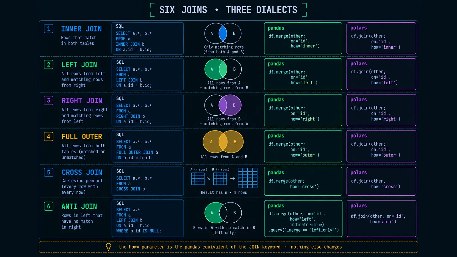
Every JOIN Type Translated

SQL has half a dozen join types. Pandas has one method — merge — and a single parameter controls the join type.

-- inner join
select * from orders o inner join customers c on c.customer_id = o.customer_id;

-- left join
select * from customers c left join orders o on o.customer_id = c.customer_id;

-- full outer
select * from customers c full outer join orders o on o.customer_id = c.customer_id;

-- cross join (cartesian)
select * from customers c cross join regions r;

# INNER JOIN — default
orders.merge(customers, on='customer_id', how='inner')

# LEFT JOIN — keep every customer, orders may be missing
customers.merge(orders, on='customer_id', how='left')

# RIGHT JOIN — same as swapping left and right
orders.merge(customers, on='customer_id', how='right')

# FULL OUTER JOIN
customers.merge(orders, on='customer_id', how='outer')

# CROSS JOIN — cartesian product
customers.merge(regions, how='cross')

Two things trip up SQL analysts.

1. Column-name collisions. If both tables have a column called region (say your customers table and a store-regions table both have one), merge() appends _x and _y suffixes by default. Cleaner: pass suffixes=('_customer', '_store'), or rename before merging.

2. Merging on differently-named keys. SQL lets you write ON a.customer_id = b.cust_id. Pandas has left_on= and right_on=:

orders.merge(
    customers.rename(columns={'customer_id': 'cust_id'}),
    left_on='customer_id', right_on='cust_id',
    how='inner',
)

The trickier join types

ANTI JOIN — "customers with no orders". SQL uses LEFT JOIN ... WHERE right.key IS NULL. Pandas uses the indicator=True parameter which flags where each row came from.

(customers
    .merge(orders, on='customer_id', how='left', indicator=True)
    .query("_merge == 'left_only'")
    .drop(columns='_merge'))

SEMI JOIN — "customers who have at least one order". SQL uses WHERE customer_id IN (SELECT customer_id FROM orders). Pandas uses .isin():

customers[customers['customer_id'].isin(orders['customer_id'])]

Range join — "orders within N days of signup". SQL joins on inequality (ON o.order_date < c.signup + interval '30 days') trivially; pandas doesn’t support inequality-only joins in merge directly. The workaround is pd.merge_asof for time-ordered joins, or DuckDB when the inequality is more complex:

# orders + closest customer signup, then filter
merged = pd.merge_asof(
    orders.sort_values('order_date'),
    customers.sort_values('signup'),
    left_on='order_date', right_on='signup',
    by='customer_id',
    tolerance=pd.Timedelta(days=30),
    direction='backward',
)

# or reach for DuckDB, which supports inequality joins natively
duckdb.sql("""
    select o.*, c.name, c.region
    from orders o
    join customers c
      on c.customer_id = o.customer_id
     and o.order_date < c.signup + interval 30 day
""").df()

The pragmatic pattern: use pandas merge for the eight cases it handles cleanly; drop into DuckDB the moment the join has inequalities, complex conditions, or multiple keys with different semantics.

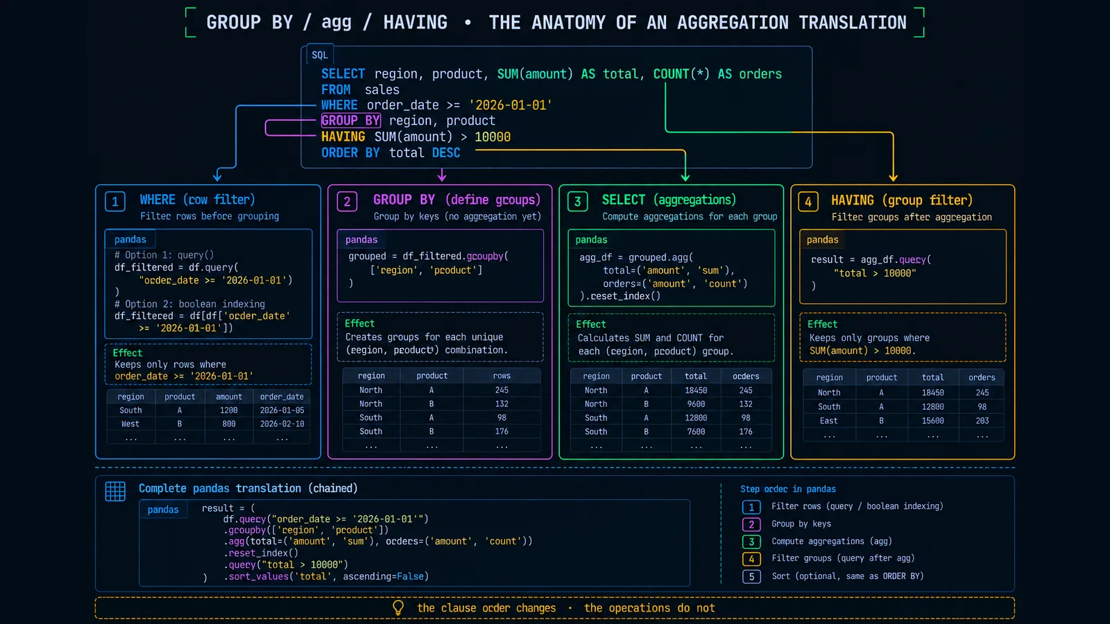
Window Functions in Pandas

SQL window functions are one of the trickier translations to pandas because pandas splits the concept across three different mechanisms: groupby().transform() for partition-scoped aggregates, groupby().cumsum()/cummax()/shift() for ordered operations, and .rolling() for frame-based windows.

For the full SQL side of window functions, see the dedicated SQL window functions post; this section is about the translation.

Ranking within a group

select
  customer_id,
  order_id,
  amount,
  row_number() over (partition by customer_id order by amount desc) as rn,
  rank() over (partition by customer_id order by amount desc) as rnk,
  dense_rank() over (partition by customer_id order by amount desc) as dnk
from orders;

o = orders.sort_values(['customer_id', 'amount'], ascending=[True, False]).copy()
o['rn']  = o.groupby('customer_id').cumcount() + 1
o['rnk'] = o.groupby('customer_id')['amount'].rank(method='min', ascending=False)
o['dnk'] = o.groupby('customer_id')['amount'].rank(method='dense', ascending=False)

The .rank() method’s method= parameter is the pandas equivalent of SQL’s tie-handling: 'min' matches SQL’s RANK, 'dense' matches DENSE_RANK, 'first' is close to ROW_NUMBER but you almost always want cumcount() for ROW_NUMBER because it’s cleaner and doesn’t need a value column to rank on.

The classic "latest row per group"

The most common window pattern in every analyst’s work: pick one row per group by some ordering.

# latest order per customer
latest = (orders
    .sort_values('order_date', ascending=False)
    .groupby('customer_id', as_index=False)
    .head(1))

# same result via drop_duplicates (usually faster on big data)
latest = (orders
    .sort_values('order_date', ascending=False)
    .drop_duplicates(subset='customer_id', keep='first'))

# or with QUALIFY-style filter after ranking
o = orders.copy()
o['rn'] = o.sort_values('order_date', ascending=False').groupby('customer_id').cumcount()
latest = o[o['rn'] == 0]

The drop_duplicates pattern is often the fastest for large data because it avoids the intermediate rank column and pandas has an optimized code path for it. For an analyst’s daily work either form is fine.

LAG and LEAD

select
  customer_id,
  order_date,
  amount,
  lag(amount, 1) over (partition by customer_id order by order_date) as prev_amount,
  lead(amount, 1) over (partition by customer_id order by order_date) as next_amount
from orders;

o = orders.sort_values(['customer_id', 'order_date']).copy()
o['prev_amount'] = o.groupby('customer_id')['amount'].shift(1)
o['next_amount'] = o.groupby('customer_id')['amount'].shift(-1)

# days since previous order (a very common analyst question)
o['prev_date'] = o.groupby('customer_id')['order_date'].shift(1)
o['days_since_prev'] = (o['order_date'] - o['prev_date']).dt.days

shift(n) is LAG. shift(-n) is LEAD. That’s the entire mapping. The sort_values before it is the pandas equivalent of the ORDER BY inside the OVER clause — without that, the shift is on physical row order, which is almost always wrong.

Running totals and moving averages

select
  order_date,
  amount,
  sum(amount) over (order by order_date rows between unbounded preceding and current row) as running_total,
  avg(amount) over (order by order_date rows between 6 preceding and current row) as mavg_7d
from orders;

o = orders.sort_values('order_date').copy()
o['running_total'] = o['amount'].cumsum()
o['mavg_7d'] = o['amount'].rolling(window=7, min_periods=1).mean()

# running total per customer (equivalent to PARTITION BY customer_id)
o['running_per_customer'] = o.groupby('customer_id')['amount'].cumsum()

.cumsum() is running total. .rolling(N) is a fixed-row-count frame. For a time-based rolling window ("last 7 days regardless of row count"), set the DataFrame index to the date and pass a string offset: o.set_index('order_date')['amount'].rolling('7D').mean().

Percentage of partition total

"This row’s amount as a percentage of the customer’s total spend" — the classic x / SUM(x) OVER (PARTITION BY customer_id).

orders['share_of_customer'] = (
    orders['amount'] /
    orders.groupby('customer_id')['amount'].transform('sum')
)

groupby().transform('sum') returns a Series with the same length and index as the input — the group aggregate is broadcast back to every row. This is the direct pandas equivalent of SQL’s window aggregate over a partition.

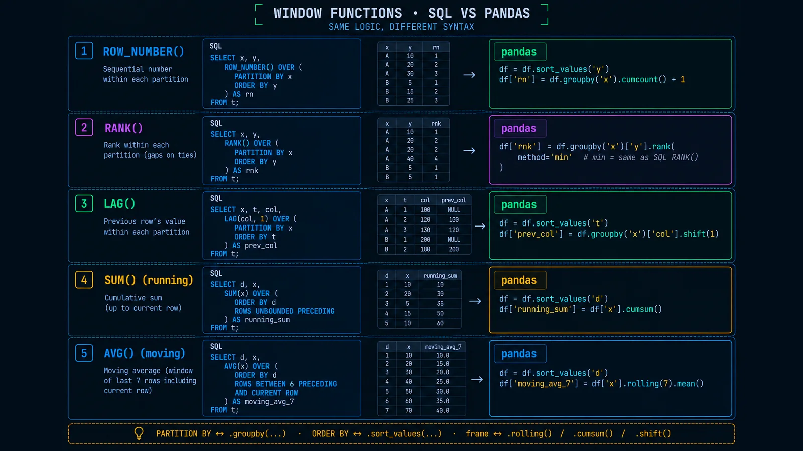
CTEs, Subqueries, and Method Chaining

Every SQL analyst uses CTEs to break a complex query into named, readable stages. Pandas does the same thing with method chaining and named intermediates — the mental model is identical, only the syntax differs.

with paid_orders as (
  select * from orders where status = 'paid'
),
customer_totals as (
  select customer_id, sum(amount) as total
  from paid_orders
  group by customer_id
),
ranked as (
  select *, rank() over (order by total desc) as rnk
  from customer_totals
)
select * from ranked where rnk <= 3;

Three good ways to translate this to pandas, in increasing readability.

Named intermediates (most CTE-like). One variable per CTE.

paid_orders     = orders[orders['status'] == 'paid']
customer_totals = paid_orders.groupby('customer_id', as_index=False)['amount'].sum().rename(columns={'amount': 'total'})
customer_totals['rnk'] = customer_totals['total'].rank(method='min', ascending=False)
top3            = customer_totals[customer_totals['rnk'] <= 3]

Method chaining (idiomatic pandas). One expression, indented for readability.

top3 = (
    orders
    .query("status == 'paid'")
    .groupby('customer_id', as_index=False)
    .agg(total=('amount', 'sum'))
    .assign(rnk=lambda d: d['total'].rank(method='min', ascending=False))
    .query('rnk <= 3')
)

.assign() deserves a call-out: it’s the pandas idiom for adding a computed column in the middle of a chain. The lambda receives the current DataFrame and returns a value for the new column. It’s the mechanism that lets you rank without breaking the chain.

Just write the SQL (DuckDB). When the CTE structure is genuinely complex, DuckDB against your DataFrames is often the readable answer.

top3 = duckdb.sql("""
    with paid_orders as (
      select * from orders where status = 'paid'
    ),
    customer_totals as (
      select customer_id, sum(amount) as total
      from paid_orders group by customer_id
    ),
    ranked as (
      select *, rank() over (order by total desc) as rnk
      from customer_totals
    )
    select * from ranked where rnk <= 3
""").df()

Analysts arriving from SQL often feel the pandas chain is less readable than a CTE. That’s partly stylistic. What helps: use named intermediates for logic and method chaining for straight-through pipelines. A 20-line chain full of .assign(lambda ...) calls is harder to read than four named CTEs and their pandas equivalents.

CASE WHEN and Conditional Logic

SQL’s CASE WHEN has three pandas translations, each with different strengths.

select
  order_id,
  amount,
  case
    when amount < 50  then 'small'
    when amount < 200 then 'medium'
    else 'large'
  end as bucket
from orders;

1. np.select — the closest to CASE WHEN in structure.

conditions = [
    orders['amount'] < 50,
    orders['amount'] < 200,
]
choices = ['small', 'medium']
orders['bucket'] = np.select(conditions, choices, default='large')

2. pd.cut — for numeric ranges specifically. Cleaner when the CASE is really a bucketing.

orders['bucket'] = pd.cut(
    orders['amount'],
    bins=[-np.inf, 50, 200, np.inf],
    labels=['small', 'medium', 'large'],
)

3. .map() or .replace() — for value lookups. Cleaner when the CASE is a direct 1-to-1 mapping.

status_display = {
    'paid':      'Completed',
    'refunded':  'Refunded',
    'cancelled': 'Cancelled',
}
orders['status_label'] = orders['status'].map(status_display).fillna('Unknown')

The .fillna('Unknown') at the end matters — .map() returns NaN for values not in the dictionary, so if you want a SQL ELSE default you fill afterwards.

4. np.where — for a single condition (SQL’s IF(cond, a, b)).

orders['is_large'] = np.where(orders['amount'] > 200, 'yes', 'no')

Rule of thumb: np.select for multi-condition, pd.cut for numeric buckets, .map for value lookups, np.where for binary flags. Every SQL CASE maps to one of these four.

String Operations

SQL’s string functions map cleanly onto pandas’ .str accessor. The accessor is what lets you call string methods vectorised across a whole column.

# UPPER / LOWER / INITCAP
customers['name'].str.upper()
customers['name'].str.lower()
customers['name'].str.title()             # INITCAP

# LENGTH
customers['name'].str.len()

# TRIM / LTRIM / RTRIM
customers['name'].str.strip()
customers['name'].str.lstrip()
customers['name'].str.rstrip()

# SUBSTRING (positions are 0-indexed in Python — SQL uses 1-indexed)
customers['name'].str.slice(0, 3)         # SUBSTRING(name, 1, 3)
customers['name'].str[:3]                  # same thing

# CONCAT
customers['name'] + ' (' + customers['region'] + ')'
customers[['name', 'region']].agg(' — '.join, axis=1)

# REPLACE
customers['region'].str.replace('APAC', 'Asia-Pacific')

# SPLIT_PART
customers['name'].str.split(' ').str[0]     # first token

# LIKE / ILIKE / REGEXP
customers['name'].str.startswith('A')
customers['name'].str.endswith('a')
customers['name'].str.contains('br', case=False, na=False)      # ILIKE %br%
customers['name'].str.match(r'^[A-D]')                          # REGEXP anchored
customers['name'].str.contains(r'^[A-D]', regex=True, na=False)  # REGEXP unanchored

# POSITION / STRPOS (1-indexed in SQL, 0 in pandas; -1 = not found)
customers['name'].str.find('a')

# LEFT / RIGHT
customers['name'].str[:2]     # LEFT(name, 2)
customers['name'].str[-2:]    # RIGHT(name, 2)

Two habits that prevent bugs. Always pass na=False to str.contains/startswith/endswith when the column can be null — without it, nulls become NaN, which breaks boolean indexing. And remember pandas is 0-indexed: str[0] is the first character, not str[1] like SQL’s SUBSTRING(x, 1, 1).

Date and Time Operations

Dates in pandas use the .dt accessor, mirroring the .str accessor for strings. Every SQL date function has a close pandas equivalent.

# parse strings to timestamps
orders['order_date'] = pd.to_datetime(orders['order_date'])

# EXTRACT / DATE_PART
orders['year']      = orders['order_date'].dt.year
orders['month']     = orders['order_date'].dt.month
orders['day']       = orders['order_date'].dt.day
orders['dow']       = orders['order_date'].dt.dayofweek   # Mon=0..Sun=6
orders['week']      = orders['order_date'].dt.isocalendar().week
orders['quarter']   = orders['order_date'].dt.quarter
orders['hour']      = orders['order_date'].dt.hour

# DATE_TRUNC
orders['month_start'] = orders['order_date'].dt.to_period('M').dt.to_timestamp()
orders['week_start']  = orders['order_date'].dt.to_period('W-MON').dt.to_timestamp()
orders['day_start']   = orders['order_date'].dt.normalize()

# DATE_ADD / DATE_SUB
orders['order_plus_7d']  = orders['order_date'] + pd.Timedelta(days=7)
orders['order_minus_1m'] = orders['order_date'] - pd.DateOffset(months=1)

# DATEDIFF
(orders['order_date'].max() - orders['order_date'].min()).days
(orders['order_date'] - customers.set_index('customer_id').loc[orders['customer_id'], 'signup'].values).dt.days

# NOW / CURRENT_DATE
pd.Timestamp.now()
pd.Timestamp.now().normalize()   # midnight today

# WHERE order_date >= CURRENT_DATE - INTERVAL 30 DAY
cutoff = pd.Timestamp.now().normalize() - pd.Timedelta(days=30)
orders[orders['order_date'] >= cutoff]

The DateOffset vs Timedelta distinction is worth internalising. Timedelta is a fixed duration (7 days is always exactly 604,800 seconds). DateOffset is calendar-aware (1 month can be 28 to 31 days). For "within 30 days" use Timedelta; for "this same date next month" use DateOffset(months=1). Choosing wrong is a source of subtle month-end bugs.

Timezones. When your source data has a timezone but pandas doesn’t know it: pd.to_datetime(col).dt.tz_localize('UTC'). When you need to convert: .dt.tz_convert('Asia/Kolkata'). Comparing a tz-aware timestamp to a tz-naive one raises TypeError — a very common source of "works locally, fails in prod" bugs.

NULL Handling

Pandas has three null representations that trip up SQL analysts: np.nan (float NaN, the historical default), pd.NA (the newer, type-agnostic missing value), and None (Python’s null). Most operations treat them equivalently, but not all.

# IS NULL / IS NOT NULL
orders['amount'].isna()
orders['amount'].notna()

# COALESCE(a, b, c) — fillna chained, or combine_first
orders['amount'].fillna(0)
orders['amount'].fillna(orders['fallback_amount']).fillna(0)   # three-arg COALESCE

# NULLIF(a, b) — turns a match into NaN
orders['amount'].where(orders['amount'] != 0)

# drop rows with any / all null
orders.dropna()                                # any null in any column
orders.dropna(subset=['amount', 'status'])   # specific columns
orders.dropna(how='all')                       # only if every col is null

Two behaviors that surprise SQL analysts.

1. NaN != NaN everywhere, including in pandas. An equality comparison against NaN is always false. Always use .isna(), never == NaN. This matches SQL’s NULL != NULL, but the syntax is different.

2. Aggregations skip nulls by default. orders['amount'].mean() matches SQL’s AVG(amount) — nulls are ignored, not treated as zero. If you need them to count as zero, fillna(0) first. If you need NaN-if-any-input-is-NaN behavior, skipna=False.

Type Conversions and Data Cleaning

SQL columns have declared types. Pandas columns have inferred types, which are correct most of the time and disastrously wrong the rest of it. A column of numbers with one stray string becomes object dtype, all arithmetic breaks, and no error message flags the moment it happened. Type discipline in pandas is what schema discipline in SQL gives you for free.

# inspect dtypes — always the first thing after a load
orders.dtypes

# CAST(x AS INTEGER)
orders['amount'].astype('int64')

# CAST(x AS FLOAT) — safer for numeric columns that may have nulls
orders['amount'].astype('float64')

# CAST(x AS VARCHAR)
orders['order_id'].astype('string')

# CAST(x AS DATE) — safest form: pd.to_datetime handles more variants
pd.to_datetime(orders['order_date'], errors='coerce')

# TRY_CAST — invalid values become NaN instead of erroring
pd.to_numeric(orders['amount'], errors='coerce')

# bulk convert on load — a lot cheaper than piecemeal astypes later
orders = orders.astype({
    'order_id':    'int64',
    'customer_id': 'int64',
    'amount':      'float64',
    'status':      'category',   # low-cardinality string
})

Three habits worth building.

1. errors='coerce' when converting from strings. Without it, one bad row (a stray "n/a" in an amount column) raises an error and halts your script. With it, that value becomes NaN and you can then investigate df[df['amount'].isna()] to see what leaked in.

2. category dtype for low-cardinality strings. A column with 5 million rows and 8 unique values (status, region, product tier) stored as object uses ~10x more memory than the same column as category. On a laptop this is often the difference between an analysis that fits and one that swaps.

3. Nullable integer types. Standard NumPy integer columns can’t hold NaN, so a merged DataFrame with unmatched rows silently upcasts your integer keys to floats. The workaround: 'Int64' (capital I) is pandas’ nullable integer type. df['customer_id'].astype('Int64') keeps integer semantics with nullability, which matches SQL’s behaviour.

Cleaning idioms

# strip whitespace from all string columns
str_cols = customers.select_dtypes(include=['object', 'string']).columns
customers[str_cols] = customers[str_cols].apply(lambda s: s.str.strip())

# normalize case
customers['region'] = customers['region'].str.upper()

# replace known bad tokens with NaN
orders = orders.replace({'amount': {'n/a': np.nan, '': np.nan}})

# rename columns to snake_case in one shot
df.columns = df.columns.str.lower().str.replace(' ', '_').str.replace('-', '_')

These are the operations every SQL analyst finds tedious in Python and then, once memorised, never has to look up again. The habit of scanning df.dtypes right after every load prevents entire classes of bug that don’t exist in SQL because the schema is declared.

UNION and Concatenation

# UNION ALL — keep all rows including duplicates
pd.concat([orders_2025, orders_2026], ignore_index=True)

# UNION — deduplicate
pd.concat([orders_2025, orders_2026], ignore_index=True).drop_duplicates()

# concat with mismatched columns — pandas fills with NaN by default
pd.concat([orders_2025, orders_2026_new_schema], ignore_index=True)

# axis=1 stitches columns side by side (rare — usually you want merge instead)
pd.concat([left_df, right_df], axis=1)

ignore_index=True is the parameter you almost always want — without it, the concatenated DataFrame keeps the original row indices from each input, which usually produces a nonsensical index.

The one gotcha: if columns differ between the frames, pandas quietly unions them, filling missing values with NaN. SQL raises an error in that case. Pandas’ permissiveness is convenient but is where schema drift between periodic loads goes unnoticed. Assert schema explicitly with set(df1.columns) == set(df2.columns) if that matters.

Pivot, Unpivot, and Crosstab

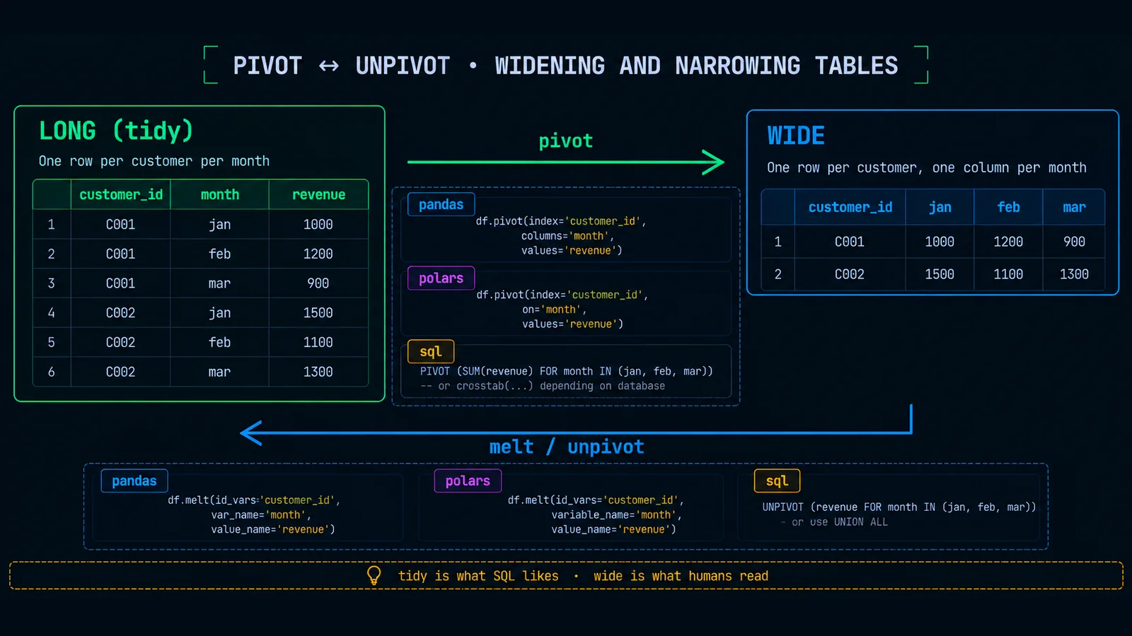
Reshaping between long and wide formats is one of the operations pandas does better than SQL — most SQL dialects require a verbose PIVOT or a manual CASE WHEN for each column. Pandas handles both directions with one method call.

Long → Wide (pivot)

# one row per customer, one column per month, values = total revenue
monthly = (orders
    .assign(month=orders['order_date'].dt.to_period('M').astype(str))
    .groupby(['customer_id', 'month'], as_index=False)
    .agg(revenue=('amount', 'sum')))

wide = monthly.pivot(index='customer_id', columns='month', values='revenue')

# with an aggregate for cases where (index, columns) has multiple rows
wide = monthly.pivot_table(
    index='customer_id',
    columns='month',
    values='revenue',
    aggfunc='sum',
    fill_value=0,
)

.pivot() requires uniqueness in the (index, columns) pair; .pivot_table() aggregates duplicates using aggfunc. Reach for pivot_table when in doubt.

Wide → Long (melt / unpivot)

long = wide.reset_index().melt(
    id_vars='customer_id',
    var_name='month',
    value_name='revenue',
)

melt is unpivot. id_vars are the columns to keep as-is; every other column is stacked into var_name / value_name. This is the operation that turns wide dashboards back into the tidy shape SQL likes.

Crosstab (a count-based pivot)

# count of orders by region × status
pd.crosstab(customers.merge(orders)['region'], orders['status'])

# with a value column and aggregate
pd.crosstab(
    index=customers.merge(orders)['region'],
    columns=orders['status'],
    values=orders['amount'],
    aggfunc='sum',
)

crosstab is a specialised pivot_table for frequency tables. It’s convenient when the aggregation is just "count how many."

Deduplication

"One row per key, keep the newest one" is the single most-run SQL query in any warehouse’s staging layer. Pandas has three ways to do it, each with a role.

# exact duplicate rows removed
orders.drop_duplicates()

# dedup by a subset of columns (default: keep first)
orders.drop_duplicates(subset=['customer_id'], keep='first')

# dedup keeping the row with the latest order_date per customer
(orders
    .sort_values('order_date', ascending=False)
    .drop_duplicates(subset=['customer_id'], keep='first'))

# dedup and count what got removed
before = len(orders)
after  = len(orders.drop_duplicates(subset=['customer_id', 'order_date']))
print(f"deduped {before - after} rows")

# find the duplicates before dropping (useful when investigating a data issue)
dupes = orders[orders.duplicated(subset=['customer_id', 'order_date'], keep=False)]
dupes.sort_values(['customer_id', 'order_date'])

The keep=False in duplicated() is worth internalising — it flags every duplicate (not just the second occurrence), which is what you want when investigating a data-quality issue. keep='first' and keep='last' flag only the ones that would be dropped.

Reading From and Writing To a Warehouse

The final piece: getting data in and out. Every Python analysis eventually needs to pull from and push to the warehouse.

import sqlalchemy as sa

# connection — the URL format varies by engine
engine = sa.create_engine("postgresql+psycopg2://user:pass@host:5432/dbname")
# snowflake+snowflake://user:pass@account/db/schema?warehouse=wh
# bigquery://project/dataset (via sqlalchemy-bigquery)

# read a table or a query into a DataFrame
df = pd.read_sql("select * from analytics.orders where order_date >= '2026-01-01'", engine)

# parametrised query (safer than string interpolation)
df = pd.read_sql(
    "select * from analytics.orders where customer_id = %(cust)s",
    engine,
    params={'cust': 101},
)

# write back — replace, append, or fail if exists
df.to_sql('my_analysis', engine, schema='sandbox', if_exists='replace', index=False)

# CSV / Parquet — file I/O
df.to_csv('output.csv', index=False)
df.to_parquet('output.parquet')
pd.read_parquet('input.parquet')

# DuckDB against a pandas DataFrame is often the fastest analysis loop
df_result = duckdb.sql("""
    select customer_id, sum(amount) as total
    from df
    where status = 'paid'
    group by customer_id
""").df()

Two habits to build. Always pass index=False to to_csv/to_sql unless you specifically want the DataFrame index written out — otherwise you get a mystery column named "Unnamed: 0" that has to be dropped every time somebody re-reads the file. And use parameterised queries (with params=) rather than f-string interpolation for user-supplied values — this is the pandas equivalent of prepared statements, and it’s how SQL injection is prevented in Python.

For everything above, DuckDB is often the fastest ramp for a SQL analyst: install it, point it at your DataFrame, and keep writing SQL. See the library comparison for when to pick which.

Common Mistakes When Coming From SQL

1. Using and/or/not in boolean expressions on columns. Use &/|/~ with parentheses. This is the #1 pandas typo for SQL analysts.
2. Forgetting to sort before shift() or cumsum(). Pandas doesn’t enforce an implicit ORDER BY — your running total will be over physical row order, which is almost never what you want.
3. Comparing == to NaN. Always NaN-false; use .isna().
4. 0-indexing vs 1-indexing. SQL’s SUBSTRING(name, 1, 3) is pandas’ name.str[:3].
5. Not passing as_index=False to groupby. The default puts the group key in the index, which breaks the next chained operation. This is one of the most-time-wasting pandas defaults.
6. Silent schema-drift in concat. SQL UNION raises an error on mismatched columns; pandas fills with NaN. Assert schema explicitly for periodic loads.
7. Not passing index=False to to_csv. The DataFrame index gets written as an unlabeled column and everyone downstream has to strip it.
8. Reading a whole table when a query would do. pd.read_sql_table pulls the entire table; pd.read_sql with a query is almost always what you want.
9. Ignoring dtypes. A column read as object when it should be int or datetime is slow and error-prone. df.dtypes after every load; convert what needs converting.
10. Chained assignment. df[df['x'] > 0]['y'] = 5 works — sometimes. It also silently fails other times, with pandas printing SettingWithCopyWarning. The safe form is df.loc[df['x'] > 0, 'y'] = 5. Never ignore SettingWithCopyWarning — it’s pointing at a bug.
11. Confusing size and count. size is COUNT(*), count is COUNT(col) (skips nulls). Picking the wrong one silently under-counts.
12. Using .apply(lambda ...) where a vectorised operation exists. .apply falls back to Python-level iteration and is 10-100x slower than the vectorised equivalent. Always look for a built-in method first.

When to Just Use SQL (via DuckDB)

Not everything is more natural in pandas. Some queries are simply cleaner in SQL, and it’s worth naming the categories where a SQL analyst should keep writing SQL rather than translating.

• Deep multi-CTE analytical queries that are easier to reason about as a query plan than as chained method calls.
• Complex joins on inequalities or on multiple conditions with OR logic.
• Analytical window functions with rare frame clauses like RANGE BETWEEN INTERVAL '7 days' PRECEDING.
• Any query where the correctness bar is higher than the ergonomics bar. SQL syntax forces you to name every column; pandas’ loose typing lets a bug hide in a mis-selected column.
• Ad-hoc joins between a DataFrame and a real warehouse table — DuckDB can query both simultaneously without you moving data around.

The pattern that keeps working: learn pandas well enough to script and glue, but reach for DuckDB the moment the transformation would be clearer as SQL. This is not a defeat — it’s the same discipline as choosing between a for-loop and a list-comprehension in ordinary Python. The right tool for the shape of the problem.

# seamless — DuckDB reads pandas DataFrames as tables in-place
import duckdb, pandas as pd

orders_df    = pd.read_csv('orders.csv')
customers_df = pd.read_csv('customers.csv')

result = duckdb.sql("""
    with paid as (
      select * from orders_df where status = 'paid'
    )
    select c.region,
           sum(p.amount) as revenue,
           count(distinct p.customer_id) as active_customers
    from paid p
    join customers_df c using (customer_id)
    group by c.region
    order by revenue desc
""").df()

Zero setup, zero connection strings, DuckDB reads your DataFrames as if they were tables. For an analyst arriving from SQL, this is often the highest-value first thing to install — more valuable than mastering pandas idioms.

Wrapping Up

Every SQL analyst who moves to Python for analysis eventually builds a personal cheat-sheet like this one — a translation table from muscle-memory SQL patterns to their pandas / polars / DuckDB equivalents. The patterns in this post cover the majority of the operations that come up in a normal analytical week: filtering, aggregation, joins, ranking, running totals, conditional logic, string and date operations, null handling, unions, pivots, deduplication, and IO.

What matters more than any single mapping is the underlying model. Pandas is imperative and column-oriented; SQL is declarative and set-oriented. The same operations are available in both; only the notation and the ordering of clauses change. Once the muscle-memory rewires — & instead of AND, .merge() instead of JOIN, .assign() instead of a SELECT column, groupby().transform() instead of window aggregates — the two languages start to feel like dialects of the same underlying analytical grammar.

The pragmatic path: use pandas for the majority of common work, drop into polars when performance matters, and drop into DuckDB whenever the query is genuinely cleaner as SQL. The three coexist happily in the same notebook. None of them is the "right" answer; the right answer is the one that produces the correct number in the fewest lines you can read a month later. See the library-comparison post for when to pick which, and the window functions deep-dive for the SQL side of the trickiest translations here.

— This article is part of an ongoing data-engineering series on techedge.in. Wrestling with any of this? Drop a comment, I read every one.