SQL Joins Explained: Every Join Type With Diagrams and Examples
INNER, LEFT, RIGHT, FULL OUTER, CROSS, and SELF joins — what each one actually does to your rows, when to reach for it, and where people get it wrong.
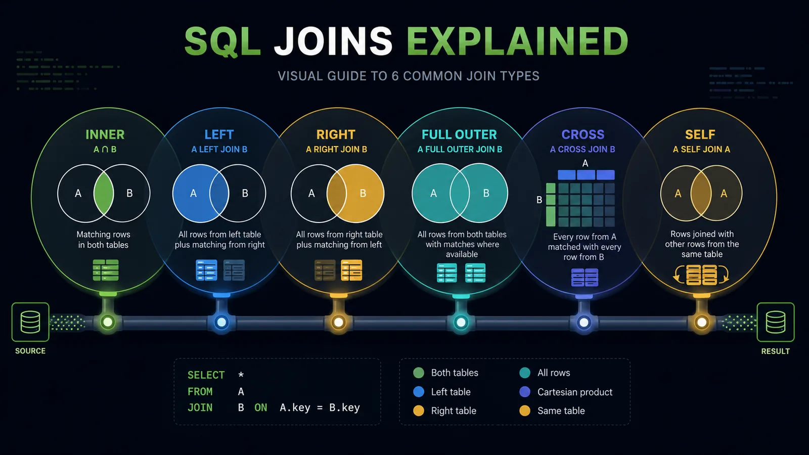
Almost every real query you write touches more than one table. Customers live in one table, their orders in another, the products those orders contain in a third — and the moment you need to answer a question that spans more than one of them, you need a join. It's one of the first things anyone learns in SQL, and also one of the things people quietly stay fuzzy on for years: the difference between a LEFT JOIN and a RIGHT JOIN is trivial once it clicks, but the difference between "why did my row count double" and "why did my row disappear entirely" usually comes down to a join misunderstanding that never got fully sorted out.
This is a practical, visual walkthrough of every join type SQL supports — what each one does to your result set row by row, when to reach for it, and where people reliably get it wrong. We'll use one small, consistent schema throughout so you can see exactly how the same two tables produce a completely different result depending on which join you pick, then cover multi-table joins, non-equality join conditions, the NULL behavior that trips people up, how joins actually execute under the hood, and a decision framework you can apply to your own queries.
What a Join Actually Does
A relational database stores data normalized — spread across separate tables to avoid repeating the same information over and over. A customers table holds each customer once; an orders table holds each order once, with a customer_id column pointing back to who placed it. That's efficient for storage and updates, but it means the answer to almost any interesting question — "which customers have never ordered," "what's the total revenue per customer," "which orders included a specific product" — doesn't live in any single table. A join is simply the operation that reassembles related rows from two or more tables into one result set, based on a condition you specify.
Conceptually, every join starts from the same place: SQL looks at every row in the first table and every row in the second table, and asks whether the join condition is true for that pair. The join type — INNER, LEFT, RIGHT, FULL, CROSS — is really just a rule about what happens to rows that don't find a match. That single idea is the thread that ties every join type in this article together, so it's worth sitting with before diving into specifics.
Sample Schema Used Throughout
To make every join type directly comparable, we'll reuse the same two small tables for every example: a handful of customers, and a handful of orders, deliberately including customers with no orders and an order pointing at a customer that no longer matches — the exact situations where join types start to diverge.
CREATE TABLE customers (
    customer_id INT PRIMARY KEY,
    name VARCHAR(100),
    city VARCHAR(100)
);

-- customer_id | name    | city
-- 1           | Asha    | Bengaluru
-- 2           | Rahul   | Mumbai
-- 3           | Meera   | Chennai
-- 4 | Farah | Delhi (no orders yet)CREATE TABLE orders (
order_id INT PRIMARY KEY,
customer_id INT,
order_total DECIMAL(10,2),
order_date DATE
);
-- order_id | customer_id | order_total | order_date
-- 101 | 1 | 1200.00 | 2026-06-01
-- 102 | 1 | 450.00 | 2026-06-14
-- 103 | 2 | 899.00 | 2026-06-20
-- 104 | 99 | 300.00 | 2026-06-22 (orphan — no matching customer)Notice the two edge cases baked in on purpose: Farah (customer_id = 4) has never placed an order, and order 104 references customer_id = 99, which doesn't exist in customers at all — a common real-world situation caused by deleted accounts, bad backfills, or referential integrity that isn't strictly enforced. Every join type below handles these two rows differently, and that's exactly the point.
INNER JOIN: Only the Rows That Match on Both Sides
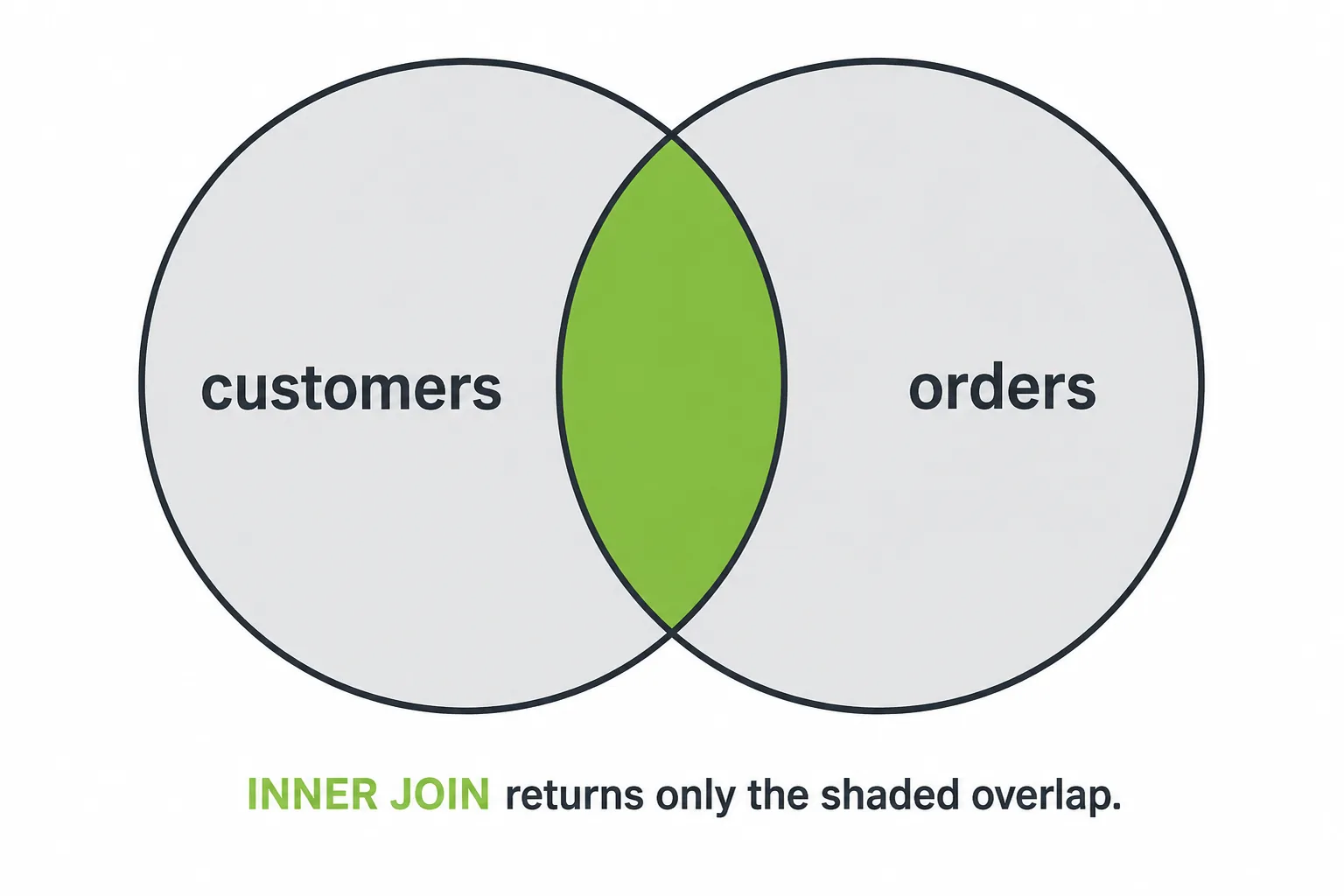
An INNER JOIN returns only the rows where the join condition finds a match in both tables. If a customer has no orders, they're excluded. If an order points at a customer that doesn't exist, that order is excluded too. It's the most restrictive join, and — not coincidentally — the one people reach for by default, since it's what plain JOIN means if you leave the keyword off.
SELECT
    c.name,
    o.order_id,
    o.order_total
FROM customers c
INNER JOIN orders o ON c.customer_id = o.customer_id;| name | order_id | order_total |
|---|---|---|
| Asha | 101 | 1200.00 |
| Asha | 102 | 450.00 |
| Rahul | 103 | 899.00 |
Meera and Farah are gone — neither has a matching row on the other side, Meera because she has zero orders, Farah for the same reason. Order 104 is gone too, since customer_id = 99 doesn't exist in customers. Three rows in, three rows out; the "no match" rows on both sides simply never make it into the result.
use it for
- Reporting on activity that must exist on both sides — revenue per customer, orders with valid product references, any query where an unmatched row is meaningless to the question being asked.
- Cleaning up orphaned or invalid references as a byproduct — an inner join naturally excludes rows with no valid match, which is sometimes exactly what you want (and sometimes a trap — see below).
- The default choice whenever you genuinely only care about rows present in both tables.
where it breaks down
The most common mistake with inner joins isn't technical, it's silent data loss. If you want "total revenue per customer, including customers with $0 in orders," an inner join will quietly drop every customer who hasn't ordered — Farah simply vanishes from the report instead of showing up with a zero. Nothing errors, nothing warns you; the row count is just smaller than you expected, and unless you're specifically checking totals against the source table, you may never notice.
LEFT JOIN: Keep Everything From the First Table
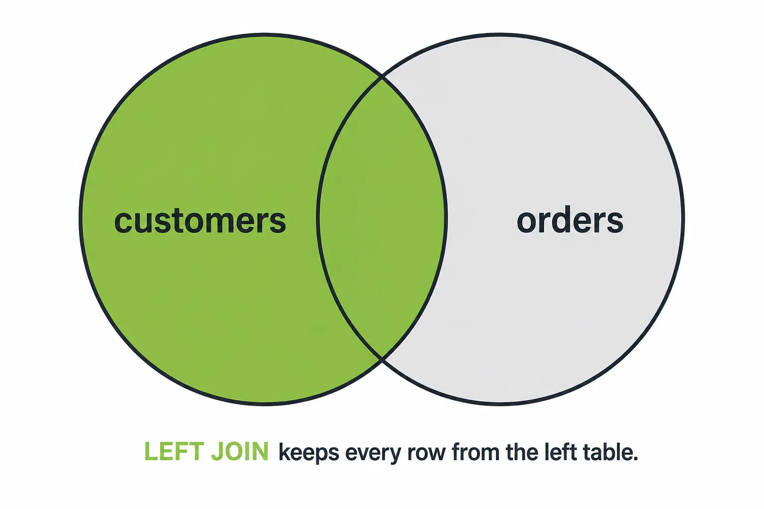
A LEFT JOIN (equivalently LEFT OUTER JOIN — the OUTER keyword is optional and rarely written out) returns every row from the left-hand table, whether or not it finds a match on the right. Where there's no match, the columns coming from the right table are filled with NULL instead of the row being dropped.
SELECT
    c.name,
    o.order_id,
    o.order_total
FROM customers c
LEFT JOIN orders o ON c.customer_id = o.customer_id;| name | order_id | order_total |
|---|---|---|
| Asha | 101 | 1200.00 |
| Asha | 102 | 450.00 |
| Rahul | 103 | 899.00 |
| Meera | NULL | NULL |
| Farah | NULL | NULL |
Every customer shows up now, including Meera and Farah, who have no orders — their order columns are simply NULL. Order 104's orphaned reference to customer_id = 99 is still gone, because 99 doesn't exist on the left side to anchor a row against. That asymmetry — the left table is fully preserved, the right table only contributes where it matches — is the entire idea behind "left."
use it for
- "All of X, with details from Y where available" queries — all customers with their most recent order, all products with their latest price change, all users with their subscription status if any.
- Finding what's missing — pair a
LEFT JOINwithWHERE right_table.key IS NULLto find rows in the left table with no match at all: customers who've never ordered, products that have never sold, users who never verified their email.
SELECT c.customer_id, c.name
FROM customers c
LEFT JOIN orders o ON c.customer_id = o.customer_id
WHERE o.order_id IS NULL;
where it breaks down
The classic mistake is putting a filter on the right-hand table's column in the WHERE clause instead of the ON clause. WHERE o.order_date >= '2026-06-01' silently turns your left join back into something that behaves like an inner join for filtering purposes, because NULL >= '2026-06-01' evaluates to unknown, which WHERE treats as false — quietly dropping the very rows (customers with no orders) you added the left join to keep. If you want to filter the right table's rows while still preserving unmatched left rows, the condition has to go in the ON clause, not WHERE.
-- WRONG: silently drops customers with zero orders
SELECT c.name, o.order_id
FROM customers c
LEFT JOIN orders o ON c.customer_id = o.customer_id
WHERE o.order_date >= '2026-06-01';

-- RIGHT: keeps all customers, filters which orders qualify
SELECT c.name, o.order_id
FROM customers c
LEFT JOIN orders o
    ON c.customer_id = o.customer_id
AND o.order_date >= '2026-06-01';RIGHT JOIN: The Mirror Image of LEFT
A RIGHT JOIN does exactly what a LEFT JOIN does, with the tables' roles reversed: every row from the right-hand table is kept, and unmatched rows from the left table are dropped, with NULLs filling in where the left table has no match.
SELECT
    c.name,
    o.order_id,
    o.order_total
FROM customers c
RIGHT JOIN orders o ON c.customer_id = o.customer_id;| name | order_id | order_total |
|---|---|---|
| Asha | 101 | 1200.00 |
| Asha | 102 | 450.00 |
| Rahul | 103 | 899.00 |
| NULL | 104 | 300.00 |
Now every order shows up, including order 104 with its orphaned customer_id, name filled with NULL because no matching customer exists. Meera and Farah, who have no orders, are gone — the same asymmetry as a left join, just flipped to the other table.
where it breaks down
In practice, RIGHT JOIN is rarely necessary on its own merit — anything you can write as a right join, you can write as a left join by swapping the table order, and most style guides prefer that for consistency and readability. It's genuinely useful when you're appending to an existing query and don't want to reorder the FROM clause, or when generated SQL (from an ORM or BI tool) produces it, but if you're writing a query from scratch, reaching for LEFT JOIN and putting the table you want fully preserved first tends to read more naturally to the next person who opens the file.
FULL OUTER JOIN: Keep Everything, From Both Sides
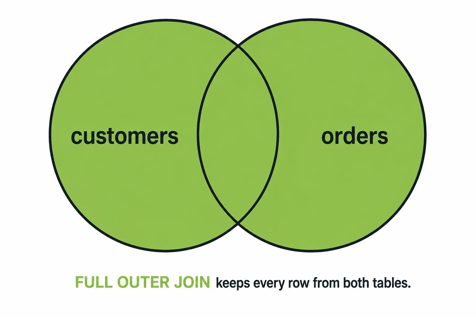
A FULL OUTER JOIN (often just written FULL JOIN) combines the behavior of LEFT and RIGHT: every row from both tables is kept, matched where possible, and NULL-padded on whichever side has no match. Nothing is dropped, from either table.
SELECT
    c.name,
    o.order_id,
    o.order_total
FROM customers c
FULL OUTER JOIN orders o ON c.customer_id = o.customer_id;| name | order_id | order_total |
|---|---|---|
| Asha | 101 | 1200.00 |
| Asha | 102 | 450.00 |
| Rahul | 103 | 899.00 |
| Meera | NULL | NULL |
| Farah | NULL | NULL |
| NULL | 104 | 300.00 |
All six logically distinct situations show up: three matched pairs, two customers with no orders, and one order with no matching customer. This is the join type to reach for when you're specifically trying to audit or reconcile two tables that are supposed to line up but might not.
use it for
- Data reconciliation — comparing two systems that should mirror each other (a source system vs a warehouse copy, an old table vs a migrated one) and surfacing every row that exists in only one side.
- Combining two independently-sourced datasets where either side might have entries the other lacks, and you don't want to lose any of them.
where it breaks down
Not every database engine supports FULL OUTER JOIN directly — MySQL notably doesn't, as of the versions most teams run in production. The standard workaround is a LEFT JOIN combined with a RIGHT JOIN via UNION, deduplicating the matched rows that would otherwise appear in both halves:
SELECT c.name, o.order_id, o.order_total
FROM customers c
LEFT JOIN orders o ON c.customer_id = o.customer_id

UNION

SELECT c.name, o.order_id, o.order_total
FROM customers c
RIGHT JOIN orders o ON c.customer_id = o.customer_id;
UNION (not UNION ALL) is what makes this work — it deduplicates the rows that matched successfully and appear identically in both halves, leaving only the unmatched rows from each side duplicated in a meaningful way, plus one copy each of the matched rows.
CROSS JOIN: Every Combination, No Condition
A CROSS JOIN is different in kind from the others: it doesn't take a join condition at all. It returns the Cartesian product — every row from the first table paired with every row from the second, regardless of whether anything matches. Three customers cross-joined with four orders produces twelve rows, not because anything relates them, but because 3 × 4 = 12.
SELECT c.name, o.order_id
FROM customers c
CROSS JOIN orders o;
-- 4 customers × 4 orders = 16 rows, every possible pairing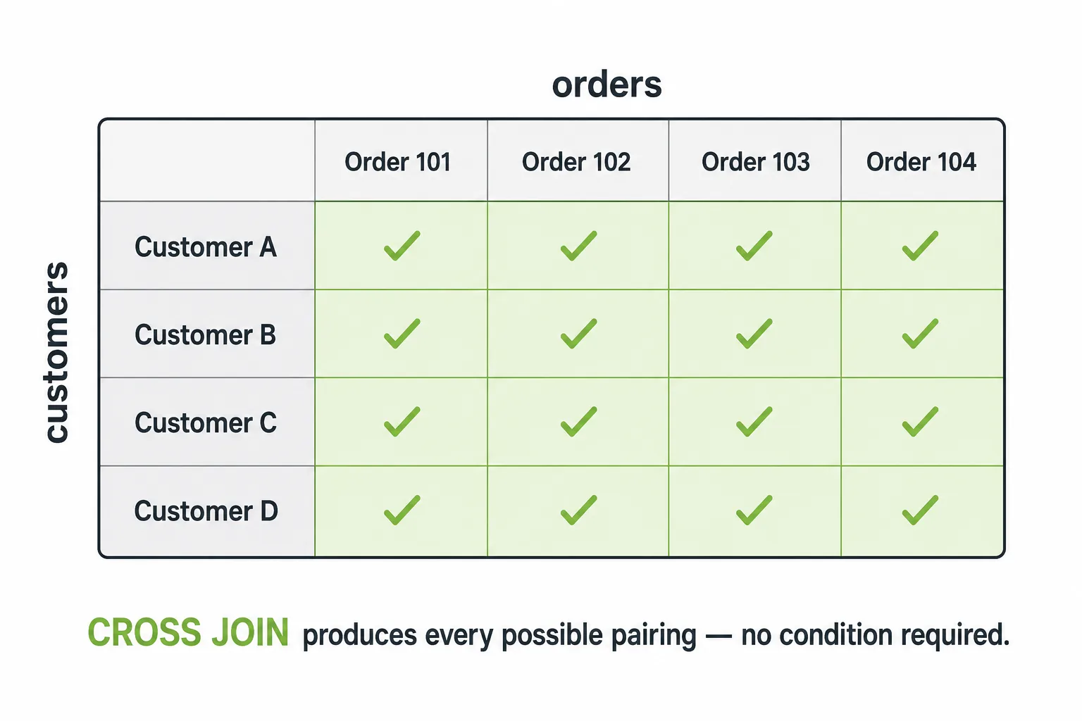
use it for
- Generating combinations deliberately — every product in every size, every store on every day of the quarter, every user against every feature flag — anywhere you need the full combinatorial set as a starting point, often filled in with actuals afterward.
- Building a date spine or number sequence to left-join real data against, so gaps (a day with zero sales, a size with zero stock) show up as explicit zero rows rather than being silently absent.
where it breaks down
The overwhelming majority of accidental cross joins aren't written on purpose — they're a missing ON clause, or a comma-separated FROM customers, orders with the join condition forgotten from the WHERE clause entirely. On small tables this fails loudly with an obviously wrong row count; on tables with tens of thousands of rows each, it can silently produce a multi-billion-row result that either crashes the query or runs for an alarmingly long time before anyone realizes what happened. If a join's row count looks like the product of the two table sizes rather than something in between, that's the signature to check for.
SELF JOIN: A Table Related to Itself
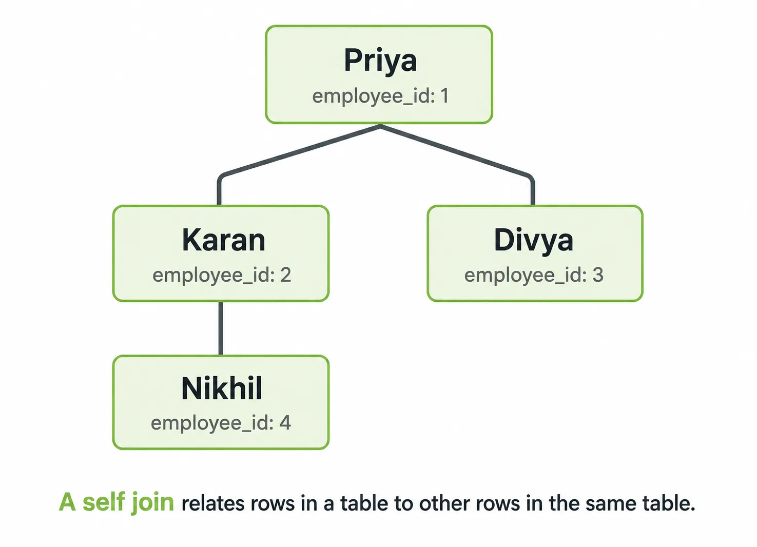
A self join isn't a distinct join type in SQL's syntax — it's an ordinary INNER or LEFT join where a table is joined to itself, given two different aliases so the query can tell "this row" from "that row." It comes up whenever rows in a table relate to other rows in the same table: employees and their managers, products and their previous-version predecessor, cities and other cities within a given distance.
CREATE TABLE employees (
    employee_id INT PRIMARY KEY,
    name VARCHAR(100),
    manager_id INT
);

-- employee_id | name    | manager_id
-- 1           | Priya   | NULL     (top of the org — no manager)
-- 2           | Karan   | 1
-- 3           | Divya   | 1
-- 4 | Nikhil | 2SELECT
e.name AS employee_name,
m.name AS manager_name
FROM employees e
LEFT JOIN employees m ON e.manager_id = m.employee_id;| employee_name | manager_name |
|---|---|
| Priya | NULL |
| Karan | Priya |
| Divya | Priya |
| Nikhil | Karan |
A LEFT JOIN is the natural choice here rather than INNER, since Priya's row would otherwise disappear entirely — an INNER self join would silently drop anyone with a NULL manager_id, which for an org chart usually means losing the person at the top.
use it for
- Hierarchies — org charts, category trees, bill-of-materials structures, any parent-child relationship stored in a single table.
- Comparing rows within the same table — finding pairs of orders from the same customer within a day of each other, matching each product to its immediate predecessor version, finding duplicate records that share a key field.
where it breaks down
Self joins only reach one level deep on their own — the query above tells you an employee's direct manager, but not their manager's manager, and can't answer "how many levels deep is this person" for an arbitrarily deep hierarchy without chaining multiple self joins (one per level) or reaching for a recursive common table expression instead, which most modern databases support via WITH RECURSIVE.
Joining Three or More Tables
Real queries rarely stop at two tables. Add a third — order_items, linking orders to the products they contain — and the pattern doesn't change, it just chains: each join clause connects the table being added to whichever table (or tables) already in the query holds the matching key.
CREATE TABLE order_items (
    order_item_id INT PRIMARY KEY,
    order_id INT,
    product_id INT,
    quantity INT
);

CREATE TABLE products (
    product_id INT PRIMARY KEY,
    product_name VARCHAR(100),
    unit_price DECIMAL(10,2)
);SELECT
c.name AS customer_name,
o.order_id,
p.product_name,
oi.quantity,
p.unit_price * oi.quantity AS line_total
FROM customers c
INNER JOIN orders o ON c.customer_id = o.customer_id
INNER JOIN order_items oi ON o.order_id = oi.order_id
INNER JOIN products p ON oi.product_id = p.product_id
ORDER BY o.order_id;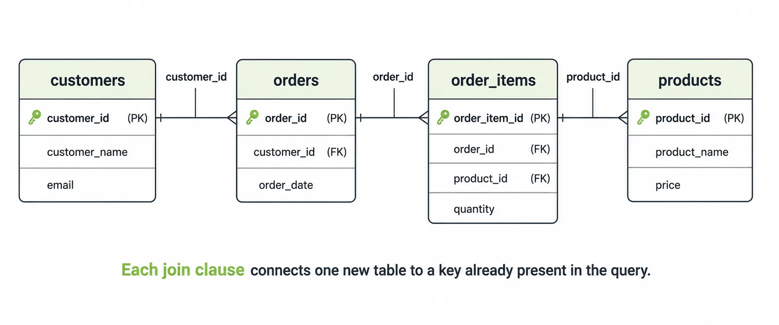
You can mix join types freely across a chain like this — perhaps INNER JOIN for orders and order_items, since a line item genuinely requires a valid order, but LEFT JOIN for a promotions table where not every order used a promo code. Each join clause is evaluated independently against the working result set built up so far, which is also why join order can matter for readability (though a good query optimizer will usually reorder physical execution regardless of how you wrote it).
One thing worth watching as chains get longer: a LEFT JOIN followed by an INNER JOIN further down the chain can silently cancel the outer join's effect. If order_items is left-joined to preserve orders with no line items, but the subsequent join to products is an inner join, any row where oi.product_id is NULL (from the unmatched left join) will fail to match products and get dropped anyway — reintroducing exactly the data loss the left join was meant to prevent. When you deliberately want to preserve unmatched rows through a chain, every join after the first outer join generally needs to stay outer too, or be written carefully with the condition in the ON clause rather than WHERE.
ON vs USING vs WHERE, and Non-Equi Joins
Every example so far has used ON table_a.key = table_b.key — an equality condition on matching column names, which covers the large majority of real joins. But the syntax and the condition itself both have more range worth knowing about.
ON vs USING
When the join columns have the identical name on both sides, USING is a shorter equivalent to a same-name ON equality, with one meaningful difference: it also collapses the two columns into a single output column instead of returning both.
-- equivalent condition, two columns named customer_id in the output
SELECT * FROM customers c JOIN orders o ON c.customer_id = o.customer_id;

-- same result rows, but a single customer_id column in the output
SELECT * FROM customers JOIN orders USING (customer_id);
USING only works when both sides genuinely share a column name, which rules it out for foreign keys named differently on each side (a common pattern: customers.id joined to orders.customer_id) — in that case ON is the only option, and in practice most teams standardize on ON everywhere for consistency rather than switching syntax based on column naming.
Non-Equi Joins
Join conditions don't have to be equality checks. Any boolean expression is valid in an ON clause, which opens up joins based on ranges, inequalities, or overlapping intervals — genuinely useful, if less common than equi-joins.
SELECT o.order_id, o.order_date, promo.promo_name
FROM orders o
INNER JOIN promotions promo
    ON o.order_date BETWEEN promo.start_date AND promo.end_date;
A classic use case is tiered pricing or bucketed classification, joining a value to whichever range row it falls within:
SELECT c.name, t.tier_name
FROM customer_totals c
INNER JOIN spend_tiers t
    ON c.total_spend >= t.min_spend
    AND c.total_spend < t.max_spend;
Non-equi joins tend to be more expensive to execute than equality joins, since the database usually can't use a simple hash or index lookup the way it can for = — see the execution section below for why that matters at scale.
WHERE-Style Implicit Joins (and Why to Avoid Them)
Older SQL, and plenty of code still in production, writes joins implicitly — listing tables comma-separated in FROM and putting the join condition in WHERE:
SELECT c.name, o.order_id
FROM customers c, orders o
WHERE c.customer_id = o.customer_id;
This produces identical results to an explicit INNER JOIN ... ON, and most optimizers handle both the same way internally, but it's worth avoiding in new code for a few concrete reasons: the join condition is separated from the tables it relates, mixing filter logic and join logic in one clause makes both harder to read at a glance, and — most importantly — there's no way to write an outer join at all in this style. It exists mostly as a compatibility note for reading legacy queries, not a pattern worth reaching for.
NULLs and Joins: The Gotchas
NULL shows up constantly around joins, in two different ways that are worth keeping separate in your head: NULLs that joins produce (covered above — unmatched rows in outer joins), and NULLs that already exist in your join keys, which behave in a way that consistently surprises people coming from general-purpose programming languages.
NULL never equals anything — not even another NULL. NULL = NULL evaluates to unknown, not true, which means a join condition can never match two NULL keys against each other.-- if both tables have a row where the join column is NULL,
-- they will NOT match each other in a standard equi-join
SELECT a.id, b.id
FROM table_a a
INNER JOIN table_b b ON a.foreign_key = b.foreign_key;
-- rows where a.foreign_key IS NULL are silently excluded,
-- even if b also has rows with a NULL foreign_keyThis matters most in two situations. First, if your foreign key column allows NULLs — an order with no assigned salesperson, a task with no assigned owner — those rows will never appear in an inner join's matched output and will always appear as unmatched in a left join, which is usually the correct behavior but worth being deliberate about rather than surprised by. Second, and more subtly: if you're deduplicating or diffing two datasets by joining on a composite key where one of the columns can be NULL, rows that are logically "the same" except for a shared NULL in one column will never match — you may need COALESCE to substitute a sentinel value before joining, or an explicit IS NOT DISTINCT FROM comparison (Postgres and a few other engines support this directly; elsewhere it has to be built by hand with OR and IS NULL checks).
-- Postgres / standard SQL:2016 IS NOT DISTINCT FROM treats NULL = NULL as true
SELECT a.id, b.id
FROM table_a a
INNER JOIN table_b b
    ON a.region IS NOT DISTINCT FROM b.region;

-- portable equivalent using COALESCE with a sentinel value
SELECT a.id, b.id
FROM table_a a
INNER JOIN table_b b
    ON COALESCE(a.region, '__none__') = COALESCE(b.region, '__none__');
How Joins Actually Execute
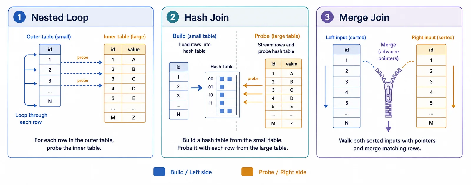
The join syntax you write is a description of the result you want, not an instruction for how to get it — the query optimizer decides the actual execution strategy, and understanding the three basic strategies it chooses between explains most of the performance behavior you'll run into.
Nested Loop Join
The conceptually simplest strategy: for every row in the outer (typically smaller) table, scan the inner table looking for matches. With no index, this is O(n × m) — genuinely the row-by-row comparison the mental model above describes. With an index on the inner table's join column, each lookup becomes fast instead of a full scan, which is why nested loop joins are usually fine, even preferred, when one side is small or an index is available — but they degrade badly as both tables grow large and unindexed.
Hash Join
For equi-joins on larger tables, most optimizers prefer building an in-memory hash table from the smaller side's join column, then scanning the larger side once, probing the hash table for each row. This is typically O(n + m) rather than O(n × m) — a large practical difference at scale — but it only works for equality conditions (hashing doesn't help for BETWEEN or >), and it needs enough memory to hold the hash table, or it spills to disk and gets considerably slower.
Merge Join
If both tables are already sorted on the join key — because of an index, or a prior sort step in the query plan — the optimizer can walk both sorted lists in a single pass, advancing whichever pointer is behind, similar to the merge step in merge sort. This is efficient and doesn't need extra memory the way a hash join does, but it depends on both inputs being sorted, which itself has a cost if neither side already is.
Reading a Query Plan
You don't have to guess which strategy your database chose — EXPLAIN (or EXPLAIN ANALYZE for actual runtime numbers, not just estimates) shows it directly:
EXPLAIN ANALYZE
SELECT c.name, o.order_id
FROM customers c
INNER JOIN orders o ON c.customer_id = o.customer_id;

-- Hash Join  (cost=1.09..2.27 rows=4 width=40) (actual time=0.02..0.03 rows=3 loops=1)
--   Hash Cond: (o.customer_id = c.customer_id)
--   ->  Seq Scan on orders o
--   ->  Hash
--         ->  Seq Scan on customers c
Two things worth checking whenever a join is slower than expected: whether the plan uses a nested loop where a hash or merge join would clearly do better (often a sign the optimizer's row-count estimates are off, sometimes fixable by updating table statistics), and whether the join columns are indexed at all — an index on a foreign key that's constantly joined against is one of the highest-leverage, lowest-effort performance changes available on most schemas, and it's surprisingly often missing, since foreign keys aren't automatically indexed the way primary keys usually are.
Common Mistakes
A handful of patterns account for most real-world join bugs, independent of the specific schema involved.
Fan-out from an unnoticed one-to-many relationship. Joining orders to order_items and then summing order_total double-, triple-, or n-tuple-counts every order with more than one line item, because the order-level total gets repeated once per matching item row. Aggregate at the correct grain first, or aggregate the child table before joining, rather than summing a parent-level column across a fanned-out join.
Filtering the outer side of a LEFT JOIN in the WHERE clause. Covered in detail above — a WHERE condition on the right-hand table's column silently turns a left join back into an inner join for filtering purposes, because unmatched rows have NULLs there, and NULL fails almost every comparison. Move the condition into the ON clause when you want to filter what matches while still keeping unmatched left rows.
An accidental CROSS JOIN from a missing or wrong join condition. A typo'd column name, a forgotten ON clause, or a comma-separated implicit join with the WHERE filter left out entirely all produce a full Cartesian product. Row counts that look like the product, rather than something in between the sizes of the two tables, are the tell.
Joining on a non-unique key without realizing it. If the "one" side of what you assumed was a one-to-many relationship actually has duplicate keys, every join against it silently multiplies rows on the other side too — the same fan-out problem as mistake #1, but from a data quality issue rather than the schema's actual cardinality.
Comparing columns with mismatched types. Joining a VARCHAR customer_id to an INT customer_id usually still "works" because of implicit type coercion, but it can silently disable index usage on that column, turning a fast indexed lookup into a full table scan — worth checking explicitly on any join that's mysteriously slow despite an index existing.
Forgetting that NULL join keys never match, including each other. Rows with a NULL in the join column will never appear as matched, in any join type — which is usually correct, but only if you've actually thought about it rather than being surprised when a row you expected to match simply doesn't.
A Decision Framework
A practical way to pick a join type for a given query:
Do you only care about rows that exist on both sides? → INNER JOIN. Simplest, and the right default when unmatched rows genuinely aren't relevant to the question.
Do you need every row from one specific table, with details from another where available? → LEFT JOIN, with that table first in the FROM clause. This is also the join to reach for when you specifically want to find what's missing — pair it with WHERE right.key IS NULL.
Do you need every row from both tables, matched where possible? → FULL OUTER JOIN — most common in reconciliation and auditing queries comparing two datasets that should, but might not, line up.
Do you need every possible combination, with no relationship between the rows at all? → CROSS JOIN, used deliberately — for generating a full combinatorial set, a date spine, or a scaffold to left-join real data onto.
Are you relating rows in a table to other rows in that same table? → a self join, aliasing the table twice, choosing INNER or LEFT per the same logic as any other join based on whether unmatched rows (like a top-level manager with no manager of their own) should be kept.
Is the relationship based on a range, inequality, or overlap rather than equality? → a non-equi join, written as an ordinary ON clause with BETWEEN, </>, or similar — just budget for it being more expensive to execute than an equivalent equality join.
When in doubt, start with INNER JOIN and a small, deliberately-constructed test case like the one used throughout this article — add a row with no match on each side, and check the row count against what you expect before trusting the query against real data. Most join bugs are cheap to catch during development and expensive to notice for the first time in a stakeholder's dashboard.
Testing Join Results
A few checks are worth running on any nontrivial join before shipping it, especially in a pipeline that runs unattended.
-- row count should match the "one" side of a one-to-many join,
-- not be inflated by unexpected duplicates on the "many" side
SELECT COUNT(*) AS joined_rows,
       (SELECT COUNT(*) FROM orders) AS source_rows
FROM orders o
INNER JOIN customers c ON o.customer_id = c.customer_id;
-- if joined_rows > source_rows, customers.customer_id isn't
-- actually unique, and this join is silently duplicating ordersSELECT COUNT(*) AS unmatched_orders
FROM orders o
LEFT JOIN customers c ON o.customer_id = c.customer_id
WHERE c.customer_id IS NULL;
-- a nonzero, unexplained count here is often the first sign
-- of an orphaned foreign key or a late-arriving dimension rowIf you're working in dbt or a similar framework, a relationships test formalizes exactly the second check — asserting that every value in a foreign key column exists in the referenced table's primary key, and failing the pipeline run if it doesn't, rather than letting an inner join quietly drop the offending rows downstream.
columns:
  - name: customer_id
    tests:
      - relationships:
          to: ref('customers')
          field: customer_id
A Realistic Query Example
Here's how several of these ideas come together in a query you might actually write against the schema used throughout this article — a per-customer revenue report that has to handle customers with no orders, avoid fan-out from multiple line items per order, and stay readable:
WITH order_revenue AS (
    -- aggregate order_items to order grain BEFORE joining,
    -- so we never fan out order_total across multiple line items
    SELECT
        o.order_id,
        o.customer_id,
        SUM(oi.quantity * p.unit_price) AS order_revenue
    FROM orders o
    INNER JOIN order_items oi ON o.order_id = oi.order_id
    INNER JOIN products p ON oi.product_id = p.product_id
    GROUP BY o.order_id, o.customer_id
)

SELECT
    c.customer_id,
    c.name,
    COUNT(r.order_id) AS order_count,
    COALESCE(SUM(r.order_revenue), 0) AS total_revenue
FROM customers c
LEFT JOIN order_revenue r ON c.customer_id = r.customer_id
GROUP BY c.customer_id, c.name
ORDER BY total_revenue DESC;
The logic, piece by piece: the CTE joins order_items to products and aggregates before anything touches the customer or order level, so a five-line-item order contributes one row, not five. The outer query then LEFT JOINs customers to that pre-aggregated revenue, specifically so that customers with zero orders — Farah, in our running example — still appear in the report, with COALESCE turning their NULL sum into an honest 0 rather than leaving a gap. INNER JOIN is correct inside the CTE, since a line item genuinely requires a valid order and product; LEFT JOIN is correct at the outer level, since the entire point of the query is to include customers who haven't ordered.
This is a reasonably common shape for real reporting queries: aggregate child data down to the right grain first, then outer-join it onto whichever table needs to be fully preserved. Getting the join type right at each stage — inner where a match is required, outer where it isn't — is usually the difference between a report that's simply correct and one that quietly under-counts.
Wrapping Up
Every join type in this article answers the same question — does this row from one table pair with a row from another — differently only in how it treats the rows that don't find a partner. INNER JOIN drops them from both sides; LEFT and RIGHT keep one side and drop the other; FULL OUTER keeps everything; CROSS skips the question of matching entirely and returns every combination; a self join is just an ordinary join pointed at the same table twice. Once that single idea is solid, the syntax differences between join types stop being things to memorize and start being an obvious consequence of what each one is for.
The practical takeaway: default to INNER JOIN when unmatched rows genuinely don't matter to the question you're asking, reach for LEFT JOIN the moment you need to preserve every row from one table — especially for "find what's missing" queries — and treat FULL OUTER and CROSS as specialized tools for reconciliation and combinatorial generation rather than everyday defaults. Watch for fan-out on one-to-many joins, keep filter conditions on outer-joined tables in the ON clause rather than WHERE, and index the foreign key columns you join on most often. Get those habits right, and most of the classic join bugs — silently missing rows, silently duplicated rows, silently exploding row counts — stop showing up in the first place.
— This article is part of an ongoing tooling series on techedge.in. Questions about a specific join you're stuck on? Drop a comment, I read every one.
One email, every other week.
New posts on data engineering, applied AI, and the business decisions around them. No noise, unsubscribe anytime.
Comments
All comments are reviewed before they appear publicly — this keeps spam out.
Loading comments…