SQL & dbt Query Optimization Techniques: Keeping Every Incremental Run Fast
A model that runs in 40 seconds on day one and eleven minutes six months later isn't unlucky — it's unoptimized. Here's what's actually going on under the hood, and the concrete techniques that keep incremental runs fast as data keeps growing.
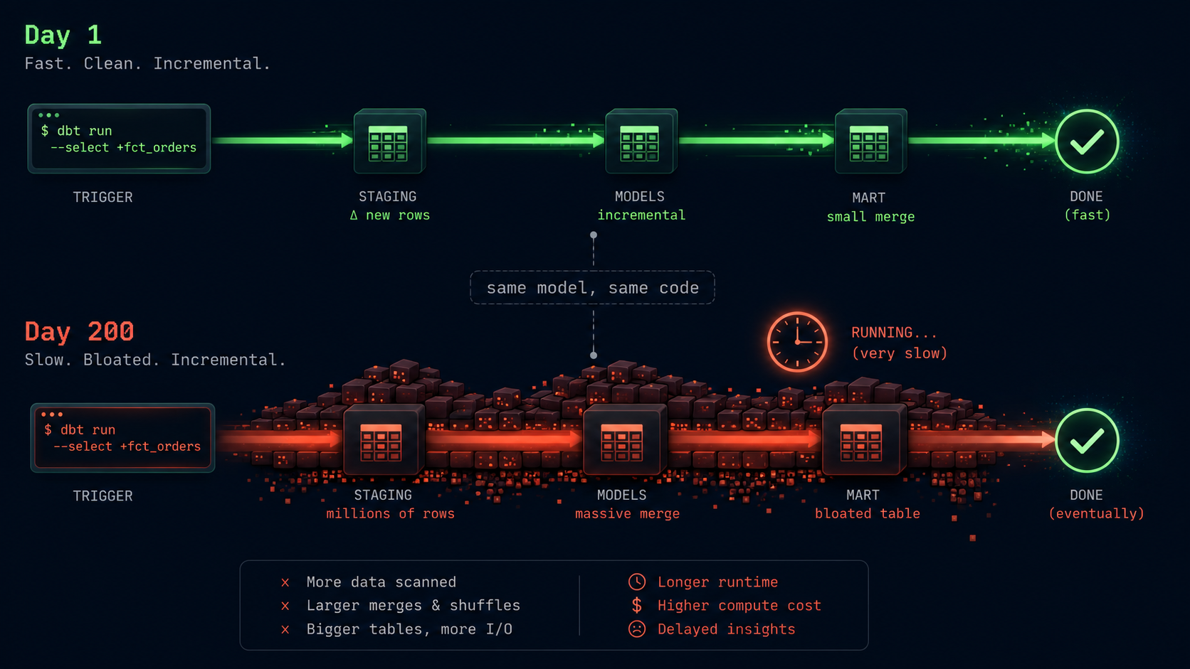
Every dbt project has a model like this somewhere. It started clean — a straightforward incremental model, a sensible unique_key, a couple of joins, done in under a minute. Nobody touched the SQL. Nobody changed the schedule. And yet, eight months later, that same model is the thing paging someone at 6 a.m. because the run window closed and it still hadn't finished. The code didn't get worse. The data did — and the query was never actually built to survive that growth in the first place.
This article is about the difference between a query that merely produces the correct answer and a query that produces the correct answer efficiently, at scale, run after run. Correctness is table stakes — dbt's testing framework, source freshness checks, and CI pipeline exist to guarantee that part. Efficiency is a separate discipline entirely, and it's the one that tends to get skipped, because a model that's "just" slow doesn't fail a test and doesn't show up in a pull request review. It just quietly gets more expensive and more fragile until someone finally has to stop and fix it under pressure.
Why This Matters More Than It Looks Like It Does
It's easy to file query optimization under "nice to have, get to it later." Three things make that filing mistake expensive in practice, and all three compound specifically with incremental models, which is why this article leans so heavily on the incremental case rather than one-off analytical queries.
First, cost. Cloud warehouses like Snowflake, BigQuery, and Databricks SQL Warehouses bill by compute consumed or bytes scanned, not by "was this query well-written." A model that scans an entire multi-terabyte fact table every run because its filter isn't sargable, or because it's missing a partition predicate entirely, pays that scan cost on every single execution — hourly, daily, however often the job runs — for as long as nobody notices. Multiply a wasteful scan by 365 runs a year and the wasted compute stops being a rounding error on the cloud bill.
Second, reliability. Every orchestration tool — Airflow, dbt Cloud, Dagster — has a run window. A model that takes 90 seconds today and 14 minutes in a year doesn't just get slower; eventually it collides with downstream dependencies, misses SLAs, or gets killed mid-run by a timeout, leaving a table in a half-updated state. Query optimization isn't just about speed for its own sake — unoptimized queries are exactly the ones that turn into 2 a.m. incident tickets once volume crosses a threshold nobody was watching for.
Third, and most specific to dbt: compounding across the DAG. A slow, unoptimized model rarely stays contained. If ten downstream models all select from one poorly filtered upstream model, that inefficiency gets paid ten times over on every full run, and it gets worse as the DAG grows — which, in any healthy dbt project, it constantly does. Optimization at the base of the DAG is leverage; optimization only at the leaf models is a much smaller, much later fix for the same underlying problem.
Why Incremental Runs Slow Down When "Nothing Changed"
The specific failure mode worth naming directly, because it's the one that catches teams off guard: an incremental model is supposed to only process new or changed rows on each run. If it's built correctly, its runtime should stay roughly flat over time — the delta being processed each run is small and bounded, regardless of how big the target table has grown. When that flatness breaks down and runtime instead grows in step with total table size, something in the model is silently behaving like a full-refresh, even though it's technically configured as incremental.
There are a small number of recurring causes, and nearly every "why did this incremental model get slow" investigation ends at one of them:
| Symptom | What's actually happening |
|---|---|
| Runtime scales with total table size, not new-row volume | The is_incremental() filter is missing, too loose, or filtering on a column the warehouse can't prune by |
| The merge step gets slower over time even though inserts stay small | The target table isn't clustered/partitioned on the merge key, so the engine has to scan broadly to find matches |
| A join that used to be instant now spills to disk | An upstream table grew past the point a join strategy (e.g. a broadcast/hash join) was designed for |
| The model itself is fast, but the whole DAG run is slow | A downstream model re-scans a full upstream table on every run, undoing the upstream model's own incremental discipline |
| Query cost creeps up with no runtime change (BigQuery, Snowflake serverless) | Bytes scanned are growing even though wall-clock time looks stable — partition pruning isn't happening |
Notice that four of these five symptoms have nothing to do with the SQL being "wrong" in the sense a test would catch — the query still returns correct results. It's the shape of the query, and its relationship to how the underlying data is physically organized, that degrades. That's the core insight this whole article is built around: optimization is mostly about aligning what your query asks for with what the engine can cheaply provide, not about clever SQL tricks.
Two Layers of Optimization: SQL and Orchestration
It helps to separate optimization into two layers, because they get fixed in different places and by different people, and conflating them is a common reason teams optimize the wrong thing first.
The SQL layer — what the query itself asks the engine to do
This is join design, filter selectivity, column pruning, window function scope, and how well your predicates line up with how the table is physically stored (partitioning, clustering). Fixing this layer means rewriting a model's SQL. It's the layer most engineers think of first when they hear "query optimization," and it's genuinely important — but it's only half the picture in a dbt project specifically.
The orchestration layer — what dbt asks the engine to do, and how often
This is materialization choice, incremental strategy, is_incremental() predicate design, DAG structure, and whether a model even needs to be recomputed on this run at all. A perfectly optimized SQL query that still gets fully recomputed every single run, when it only needed the last day's data, is still wasteful — the SQL layer alone can't fix an orchestration-layer problem.
Most of the high-leverage fixes in this article live in the second layer, precisely because that's the layer that's specific to dbt and specific to incremental workloads, and it's the layer that's easiest to overlook if you're thinking about optimization purely as "write faster SQL."
Read the Query Plan Before You Touch Anything
The single most common mistake in query optimization isn't writing bad SQL — it's optimizing based on a guess instead of evidence. Every major warehouse exposes a query plan or profile: EXPLAIN in Postgres/Redshift, the Query Profile in Snowflake, the execution details panel in BigQuery, the Spark UI's SQL tab in Databricks. Before rewriting anything, that plan answers the only question that actually matters: where is the time and the data volume actually going?
EXPLAIN ANALYZE
SELECT *
FROM analytics.fct_orders
WHERE order_date >= current_date - INTERVAL '3 days';
What you're looking for, specifically: whether a partition or clustering key is actually being pruned (most engines will explicitly show "partitions scanned: 3 of 400" or similar), whether a join is broadcasting a large table instead of a small one, whether a sort or aggregation is spilling to disk, and which single step in the plan is consuming the disproportionate share of the total time or bytes scanned. It's very common for a query with five joins to have four of them be essentially free and one be responsible for 90% of the cost — and no amount of tuning the other four will move the needle if that one join is left untouched.
1. Partition Pruning & Predicate Pushdown
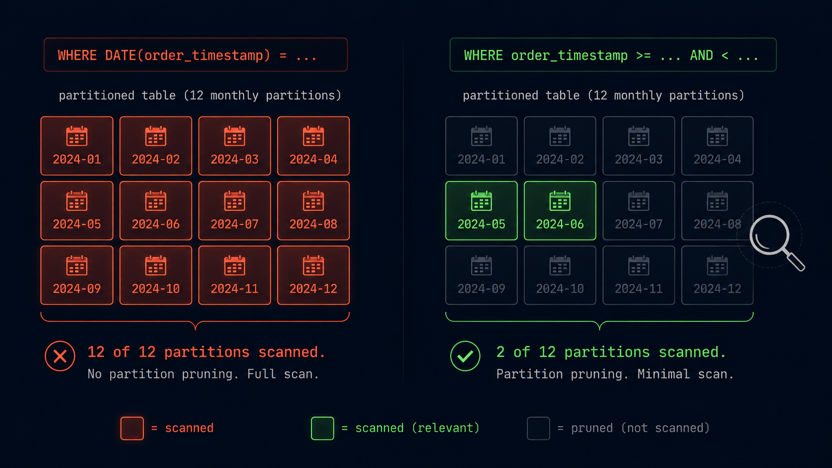
This is the single highest-leverage technique in this entire article, and it's the one most incremental models get subtly wrong. Modern warehouses store large tables physically divided into partitions (BigQuery's partitioned tables, Snowflake's micro-partitions plus clustering keys, Redshift's sort keys, Databricks/Delta's file-level partitioning). When a query's WHERE clause filters on the partitioning column in a way the engine can statically understand, it skips reading the partitions that can't possibly match — this is partition pruning, and it's the difference between scanning 3 days of data and scanning 3 years of data for the exact same logical result.
The trap is that pruning only works when the filter is "sargable" — expressed in a form the engine's planner can evaluate against partition metadata before reading any rows. Wrapping the partition column in a function is the most common way to accidentally defeat this.
SELECT *
FROM fct_orders
WHERE DATE(order_timestamp) = '2026-08-01';
-- the engine can't check partition metadata against DATE(order_timestamp)
-- without first computing it row by row — every partition gets scannedSELECT *
FROM fct_orders
WHERE order_timestamp >= '2026-08-01'
AND order_timestamp < '2026-08-02';
-- a plain range comparison on the raw column lets the engine
-- check partition min/max metadata and skip non-matching partitions entirelyThe same principle applies to type casts, string manipulation, and coalesce logic on partition or clustering columns — anything that turns a direct comparison into "compute something, then compare" tends to force a full scan. This one habit — always filter on the raw column, in its native type, with a plain comparison — accounts for a disproportionate share of "why is this suddenly scanning everything" incidents.
2. Tight, Correct Incremental Predicates
This is the orchestration-layer twin of partition pruning, and it's specific to dbt's is_incremental() macro. The entire performance promise of an incremental model rests on this filter being both correct and tight — correct so you don't silently drop late-arriving data, and tight so you're not accidentally reprocessing far more history than the model actually needs.
{{
  config(
    materialized='incremental',
    unique_key='order_id',
    incremental_strategy='merge'
  )
}}

SELECT
    order_id,
    order_status,
    order_total,
    updated_at
FROM {{ source('raw', 'orders') }}

{% if is_incremental() %}
  WHERE updated_at >= (
    SELECT dateadd('day', -3, max(updated_at)) FROM {{ this }}
  )
{% endif %}
The 3-day lookback here isn't arbitrary caution — it's a deliberate design decision that handles late-arriving data (a row that gets updated a day after it was first inserted) without needing to rescan the entire table's history to find it. Too short a window and you silently lose legitimately late updates; too long a window and you're back to scanning far more than necessary on every run, quietly recreating the exact problem incremental models exist to solve. The right window width is a business question — how late does data from this source realistically arrive — not a technical one, which is exactly why it's so often left as an untuned default.
A second, subtler version of this same mistake: filtering on {{ this }} without an index-friendly comparison. SELECT max(updated_at) FROM {{ this }} is itself a query, and if the target table isn't clustered on that column, even that lookup can be expensive on a large table — you can end up paying a full scan just to figure out where the incremental window should start.
3. Choosing the Right Materialization for the Workload
Materialization choice is itself a performance decision, not just a modeling-style one. A view recomputes its logic on every single downstream query — fine for something queried rarely, actively wasteful for something hit by a BI dashboard hundreds of times a day. A table trades storage and build time for fast reads. An incremental model trades some complexity for keeping both build time and storage growth bounded as the source keeps growing. Getting this choice wrong in either direction has a performance cost, just paid in different places.
| Materialization | Where the performance cost lands | Right fit |
|---|---|---|
| View | Every downstream query re-runs the full logic | Rarely queried, cheap logic, staging-layer thin wrappers |
| Table | Every dbt run, full rebuild cost | Small-to-medium tables, or logic too complex/expensive to re-derive per query |
| Incremental | Build cost bounded by delta size, but adds merge/predicate complexity | Large, append-or-update-heavy fact tables that grow continuously |
| Ephemeral | Inlined as a CTE into every downstream model that references it | Small, single-purpose logic reused by exactly one or two downstream models |
The ephemeral row is worth a specific warning: an ephemeral model isn't "free" just because it doesn't materialize its own object. Its SQL gets inlined as a CTE into every downstream model that references it, at every level. Reference an ephemeral model from five different downstream models, and its logic — including any expensive joins or aggregations inside it — gets recompiled and re-executed five separate times, once per downstream query, rather than computed once and reused. For anything nontrivial referenced by more than one or two models, a view or table is almost always the better performance trade, even though it's the less "clever" choice.
4. Matching Incremental Strategy to Its Real Cost
dbt's incremental strategies — append, merge, delete+insert, insert_overwrite, microbatch — aren't interchangeable on performance, even when they produce identical logical results. Each one issues fundamentally different SQL under the hood, and picking the wrong one for your data pattern is a common, avoidable source of slow runs.
append is the cheapest possible operation — a plain insert, no scan of the existing target table required at all. It's also the least safe: it has no way to prevent duplicates if a row gets reprocessed, so it only belongs on genuinely append-only data (immutable event logs, for instance). merge is more expensive because it has to locate matching rows by unique_key across the entire (or clustering-pruned) target table, but it's correct for mutable data. insert_overwrite, where supported, sidesteps row-level matching entirely by replacing whole partitions — often meaningfully cheaper than a row-level merge when your data is naturally partitioned by date and a given day's partition might legitimately need to be reprocessed wholesale.
merge pays a real, avoidable matching cost on every run for a guarantee it never needed.5. Clustering & Physical Table Design
Partition pruning gets a table down to the right day or range. Clustering (Snowflake's clustering keys, BigQuery's clustering columns, Redshift's sort/dist keys, Delta's Z-ordering) gets it further — organizing data physically so that rows likely to be filtered or joined together are stored near each other on disk, so even within a pruned partition, the engine reads less.
The mistake most teams make here isn't skipping clustering entirely — it's clustering on the wrong column, usually chosen by intuition ("we filter on customer_id a lot") rather than by looking at what queries actually run against the table. A good clustering key is high-cardinality enough to be selective, but matches the columns that show up in WHERE clauses and join predicates most frequently — which for most fact tables ends up being a date column, sometimes paired with a second dimension like region or tenant_id.
ALTER TABLE analytics.fct_orders
CLUSTER BY (order_date, region);
Two practical notes that get missed often enough to be worth stating directly. First, clustering isn't free to maintain — the warehouse does ongoing background work to keep a large, frequently-updated table well-clustered, and that has its own cost, so it's worth reserving for tables that are genuinely large and genuinely frequently queried, not applying reflexively to every model. Second, re-clustering after a bulk backfill or full-refresh is easy to forget — a table clustered well on day one can drift out of good physical order after a large one-off load, quietly degrading query performance until someone notices and re-clusters it.
6. Writing Joins the Engine Can Actually Optimize
Join order and join type matter less than most people assume on modern cost-based-optimizer warehouses — Snowflake, BigQuery, and Databricks will all reorder joins based on statistics, not strictly the order you wrote them in. What matters far more is giving the optimizer accurate, filterable inputs to work with in the first place.
The most consequential join-design decision is filter placement: filtering each table down to only the rows you need before the join, rather than joining everything and filtering afterward. This sounds obvious stated plainly, but it's routinely violated in dbt projects built up through layered ref() chains, where a downstream model joins two upstream models that were each already selected in full, with the actual narrowing filter tacked on at the very end.
WITH orders AS (
    SELECT * FROM {{ ref('stg_orders') }}
),
customers AS (
    SELECT * FROM {{ ref('stg_customers') }}
)
SELECT o.*, c.customer_name
FROM orders o
JOIN customers c ON o.customer_id = c.customer_id
WHERE o.order_date >= current_date - INTERVAL '3 days';WITH orders AS (
SELECT * FROM {{ ref('stg_orders') }}
WHERE order_date >= current_date - INTERVAL '3 days'
),
customers AS (
SELECT * FROM {{ ref('stg_customers') }}
)
SELECT o.*, c.customer_name
FROM orders o
JOIN customers c ON o.customer_id = c.customer_id;Most modern optimizers can push a trailing predicate back through a simple CTE automatically — but that predicate pushdown isn't guaranteed once the CTE involves aggregation, a window function, or a UNION, and relying on the optimizer to do it for you is a bet, not a guarantee. Filtering explicitly and early costs nothing and removes the bet entirely.
The second consequential decision is join key types matching. A join between an INT column and a VARCHAR column, or between two differently-precisioned numeric types, forces an implicit cast on every row of the larger side before the join can even be evaluated — invisible in the SQL, expensive in the execution plan. Keeping key types consistent across a model's sources is a small modeling discipline with an outsized payoff on large joins.
7. Avoiding Join Fan-Out
Fan-out happens when a join's "many" side isn't as unique as the model assumes, silently multiplying row counts — and, downstream, multiplying every aggregate built on top of that join. It's one of the more dangerous performance-and-correctness issues at once, because a fanned-out join doesn't error; it just quietly processes far more rows than intended and can produce wrong numbers alongside the wasted compute.
SELECT
    o.order_id,
    o.order_total,
    count(oi.item_id) AS item_count
FROM orders o
JOIN order_items oi ON o.order_id = oi.order_id
GROUP BY 1, 2;
-- if a promotions table is joined in later without a 1:1 relationship
-- to orders, every order row silently multiplies by the number of
-- matching promotion rows -- both row count and aggregate scale blow up
Guarding against this is mostly about explicit assumptions, not clever SQL: a dbt_utils.unique_combination_of_columns test (or an equivalent uniqueness check) on the join key of the "one" side of any intended one-to-many relationship, run in CI, catches a fan-out before it ships rather than after someone notices revenue numbers doubled. It's also worth pre-aggregating the "many" side into its own CTE or intermediate model before joining, rather than joining raw and aggregating afterward — that makes the intended cardinality explicit in the code itself, and gives the optimizer a smaller, pre-shrunk input to work with.
8. Taming Expensive Window Functions
Window functions are indispensable for change detection, deduplication, and running totals — and they're also one of the easiest ways to accidentally force a full, unpartitioned sort across an entire large table. The cost of a window function is driven almost entirely by its PARTITION BY and ORDER BY clauses: a wide, low-cardinality partition key forces the engine to sort huge groups of rows together.
WITH recent_orders AS (
    SELECT * FROM {{ ref('stg_orders') }}
    WHERE order_date >= current_date - INTERVAL '3 days'
),
deduped AS (
    SELECT *,
        row_number() OVER (
            PARTITION BY order_id
            ORDER BY updated_at DESC
        ) AS rn
    FROM recent_orders
)
SELECT * FROM deduped WHERE rn = 1;
The pattern worth internalizing: run the window function against the smallest input you can, not against the full table with a filter applied afterward. This is the same "filter before you do the expensive thing" principle from the join section, applied to sorts instead of joins — and it matters even more here, because a window function's sort cost tends to scale worse than a simple filtered scan does as row count grows.
9. Column Pruning & the Real Cost of SELECT *
On columnar warehouses — which is most modern cloud warehouses — a query only reads the columns it actually references, not entire rows. That makes SELECT * more than a style preference: on a wide table with 80 columns, selecting all of them when a downstream model only needs six means paying for I/O and network transfer on 74 columns nobody will use. This compounds specifically in layered dbt projects, where a wide staging model gets selected from in full by three intermediate models, each of which gets selected from in full again by marts on top — the same unused columns get paid for repeatedly, at every layer.
The practical fix isn't retyping every column list by hand — that's what dbt_utils.star() exists for, letting you select everything except a documented exclusion list, or conversely, defining an explicit, intentional column list at the staging layer that every downstream model inherits. Either approach beats a bare SELECT * propagating unexamined through five layers of the DAG.
10. CTEs, Ephemeral Models, and Where Query Flattening Bites
Most warehouses today either fully inline CTEs into the surrounding query or materialize them as lightweight temporary results — either way, a chain of CTEs referencing each other isn't automatically expensive on its own. Where this becomes a real performance issue is specifically the ephemeral-model case already flagged above: unlike a CTE within one model's own SQL file, an ephemeral dbt model gets its entire compiled SQL re-inlined into every downstream model that calls ref() on it, at compile time, before the query ever reaches the warehouse.
The practical implication for large or deeply layered dbt projects: keep an eye on how many downstream models reference each ephemeral model, and don't be shy about promoting one to a view or table the moment more than a couple of models depend on it. This is a case where a small dbt-specific mental model — "ephemeral means duplicated, not means free" — prevents a real, easy-to-miss performance regression that has nothing to do with the SQL's own logic being wrong.
11. Optimizing at the DAG Level, Not Just the Model Level
Everything above optimizes a single model in isolation. The highest-leverage optimizations in a mature dbt project, though, often live one level up — in how models relate to each other across the DAG.
The most common DAG-level waste: an upstream model is correctly incremental and processes only the last 3 days of data efficiently — but a downstream model built on top of it does SELECT * FROM {{ ref('upstream_model') }} with no filter of its own and is materialized as a full-refresh table. Every run, that downstream model quietly reprocesses the upstream model's entire history, undoing the upstream model's own incremental discipline for the purposes of anything built on top of it. The upstream model looks fast in isolation; the actual end-to-end pipeline is not.
The fix is usually to make the downstream model incremental too, with its own predicate mirroring the upstream lookback window — propagating the "only touch recent data" discipline all the way through the DAG rather than letting it dead-end at the first model that happens to be marked incremental. dbt's dbt ls --select +model_name and the lineage graph in dbt docs are the fastest way to actually see which downstream models are quietly undoing an upstream model's incremental design.
12. Running Tests Without Tanking Run Performance
Data quality tests matter — nothing in this article argues otherwise — but tests themselves are queries, and an inefficient test suite can add meaningful time to every single CI run and scheduled job. A unique or not_null test on a large table, run against the entire table on every single execution rather than just the newly changed rows, is a common and avoidable source of slow test suites.
dbt's store-failures and limit-based test configs help here directly — capping how many failing rows a test materializes, and, for incremental models specifically, scoping expensive tests to run only against recently changed data using the same lookback-window pattern used in the model itself, rather than re-validating the full historical table on every run once it's already been validated in a prior run.
models:
  - name: fct_orders
    columns:
      - name: order_id
        tests:
          - unique:
              config:
                where: "order_date >= dateadd('day', -7, current_date)"
13. Monitoring, Query History, and Finding the Real Bottleneck
Everything in this article assumes you can actually see which model or which query step is the problem, and that requires monitoring, not memory. Most warehouses expose a queryable history table — Snowflake's QUERY_HISTORY, BigQuery's INFORMATION_SCHEMA.JOBS, Redshift's STL_QUERY — that can be joined back to dbt's own run metadata (via query tags or dbt's invocation_id) to answer, concretely and with numbers, "which models got slower, and when."
SELECT
    query_tag,
    query_text,
    total_elapsed_time / 1000 AS seconds,
    bytes_scanned
FROM snowflake.account_usage.query_history
WHERE query_tag LIKE 'dbt%'
  AND start_time >= dateadd('day', -30, current_timestamp())
ORDER BY seconds DESC
LIMIT 20;
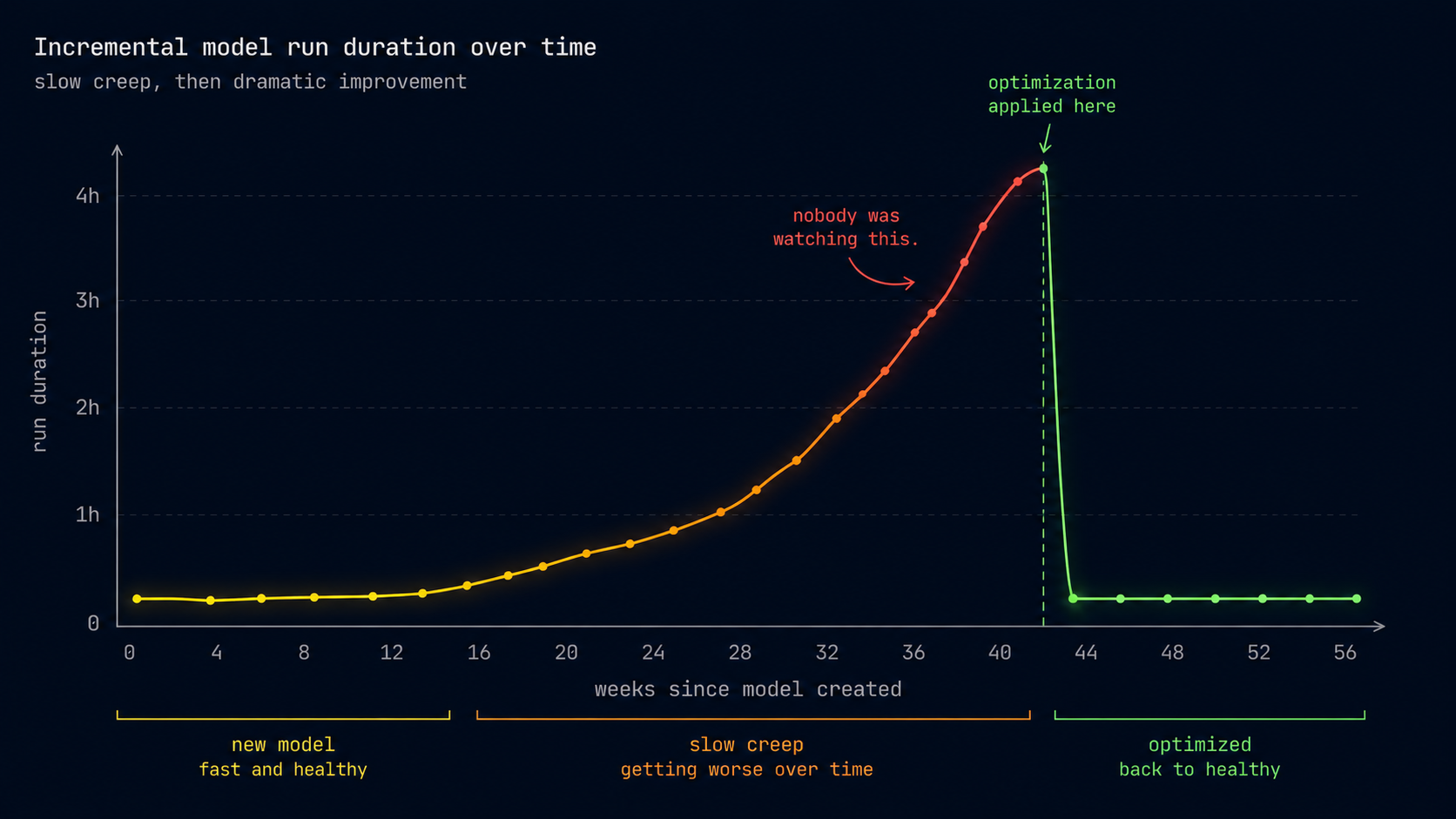
Trending this over time — not just looking at it once — is what actually catches the "slow creep" failure mode from earlier in this article, well before it turns into a missed SLA. A model that's grown from 40 seconds to 90 seconds over three months is a five-minute fix today; the same model at 14 minutes, discovered only once it starts blowing through the run window, is a much more stressful fix under time pressure.
A Worked Example, Start to Finish
To make this concrete rather than abstract, here's a realistic before-and-after on a single model — a fct_order_events incremental model that started fast and degraded over roughly six months as the underlying event table grew from around 2 million to over 400 million rows.
{{ config(materialized='incremental', unique_key='event_id') }}

SELECT
    e.*,
    DATE(e.event_timestamp) AS event_date,
    c.customer_tier
FROM {{ source('raw', 'events') }} e
JOIN {{ ref('dim_customers') }} c ON e.customer_id = c.customer_id

{% if is_incremental() %}
  WHERE DATE(e.event_timestamp) >= (SELECT max(event_date) FROM {{ this }})
{% endif %}
Three separate problems were stacked in this one model, each individually small, together responsible for the slow creep. The DATE(e.event_timestamp) wrapper defeated partition pruning on the raw source, forcing a full scan of the event table on every run regardless of the filter's intent. The join against dim_customers pulled every column with no upstream narrowing, widening the scan further. And the lookback used max(event_date) from the target with no buffer window at all, meaning any event that arrived even slightly late — a common pattern with event pipelines — was silently dropped rather than caught on a later run.
{{ config(
    materialized='incremental',
    unique_key='event_id',
    incremental_strategy='merge'
) }}

WITH recent_events AS (
    SELECT
        event_id, customer_id, event_type, event_timestamp,
        DATE(event_timestamp) AS event_date
    FROM {{ source('raw', 'events') }}
    {% if is_incremental() %}
      WHERE event_timestamp >= (
        SELECT dateadd('day', -2, max(event_timestamp)) FROM {{ this }}
      )
    {% endif %}
),
customers AS (
    SELECT customer_id, customer_tier FROM {{ ref('dim_customers') }}
)
SELECT re.*, c.customer_tier
FROM recent_events re
JOIN customers c ON re.customer_id = c.customer_id;
The fixes: filter on the raw event_timestamp instead of a computed DATE() wrapper, so partition pruning actually engages; narrow dim_customers to just the two columns actually needed before the join; and add a genuine two-day lookback window instead of a bare "since max" filter, so late-arriving events get caught on the next run rather than silently dropped. None of these are individually exotic — that's the point. Runtime on this model went from a steadily climbing 11 minutes back down to a flat, sub-90-second run, and stayed flat as the table kept growing, because the fixes addressed the actual scaling behavior rather than just the current symptom.
Common Mistakes That Quietly Kill Performance
Wrapping the partition/filter column in a function. DATE(), CAST(), string concatenation, or COALESCE applied to the column you're filtering on defeats partition pruning almost every time — filter on the raw column in its native type instead.
An incremental model with no real lookback window. A bare "since max(updated_at)" filter either drops late-arriving data silently or, if made too generous "just in case," quietly reprocesses far more than necessary every single run.
Treating an ephemeral model as free. Its logic gets recompiled and re-executed once per downstream reference — cheap for one consumer, expensive once several models depend on it.
Filtering after a join instead of before it. Especially once a CTE involves aggregation or a window function, predicate pushdown through it isn't guaranteed — filter each input explicitly before the join, don't rely on the optimizer to figure it out.
Optimizing one model while its downstream consumers undo the work. An efficient, tightly-filtered incremental model feeding a downstream full-table-scan model has fixed nothing end-to-end — check the DAG, not just the model in front of you.
A Practical Optimization Checklist
Before calling a model "optimized," check these
- Does the query plan actually show partition pruning happening, or is a full scan hiding behind a filter that looks correct?
- Is the
is_incremental()predicate filtering on a raw column, with a deliberate lookback window sized to your data's real lateness? - Is the table clustered or partitioned on the column(s) actually used in
WHEREclauses and join keys — not just the column that felt intuitive? - Are joins filtered down on both sides before the join executes, not after?
- Is any ephemeral model referenced by more than one or two downstream models — and if so, should it be a view or table instead?
- Do downstream models preserve the incremental discipline of their upstream sources, or does a full-refresh model quietly re-scan everything?
- Are tests scoped to recent data where the model itself is incremental, instead of re-validating full history every run?
- Is there an actual dashboard or query trending run duration and bytes scanned over time, or would a regression only get noticed once it breaks an SLA?
The Bottom Line
Almost none of the techniques in this article are exotic. Filter on raw columns. Give incremental models a real, deliberate lookback window. Narrow inputs before joins and window functions, not after. Cluster tables on the columns you actually query by. Check what's happening downstream, not just in the model you're staring at. None of it requires a rewrite in a different language or a fundamentally different architecture — it requires treating query shape and data growth as a first-class design concern from the start, rather than a cleanup task that gets scheduled once a model is already slow enough to hurt.
The uncomfortable part is that most of this is invisible until it isn't. A model that's technically correct and mildly inefficient looks identical to a model that's correct and well-optimized, right up until data volume crosses whatever threshold turns "a little wasteful" into "blowing through the run window." The teams that don't get paged for this build the habit of checking query plans and lookback windows into how they write models in the first place — not as a separate performance pass bolted on after something breaks, but as part of what "done" means for an incremental model from day one.
— This article is part of an ongoing tooling series on techedge.in. Got a specific model that's crept from fast to slow and can't figure out why? Drop the details in a comment — happy to help think through the query plan.
One email, every other week.
New posts on data engineering, applied AI, and the business decisions around them. No noise, unsubscribe anytime.
Comments
All comments are reviewed before they appear publicly — this keeps spam out.
Loading comments…