CTEs vs. Subqueries vs. Temp Tables: When to Use Which
Three ways to break a query into pieces — what each one actually costs in readability, performance, and debuggability, and a straightforward way to decide between them.
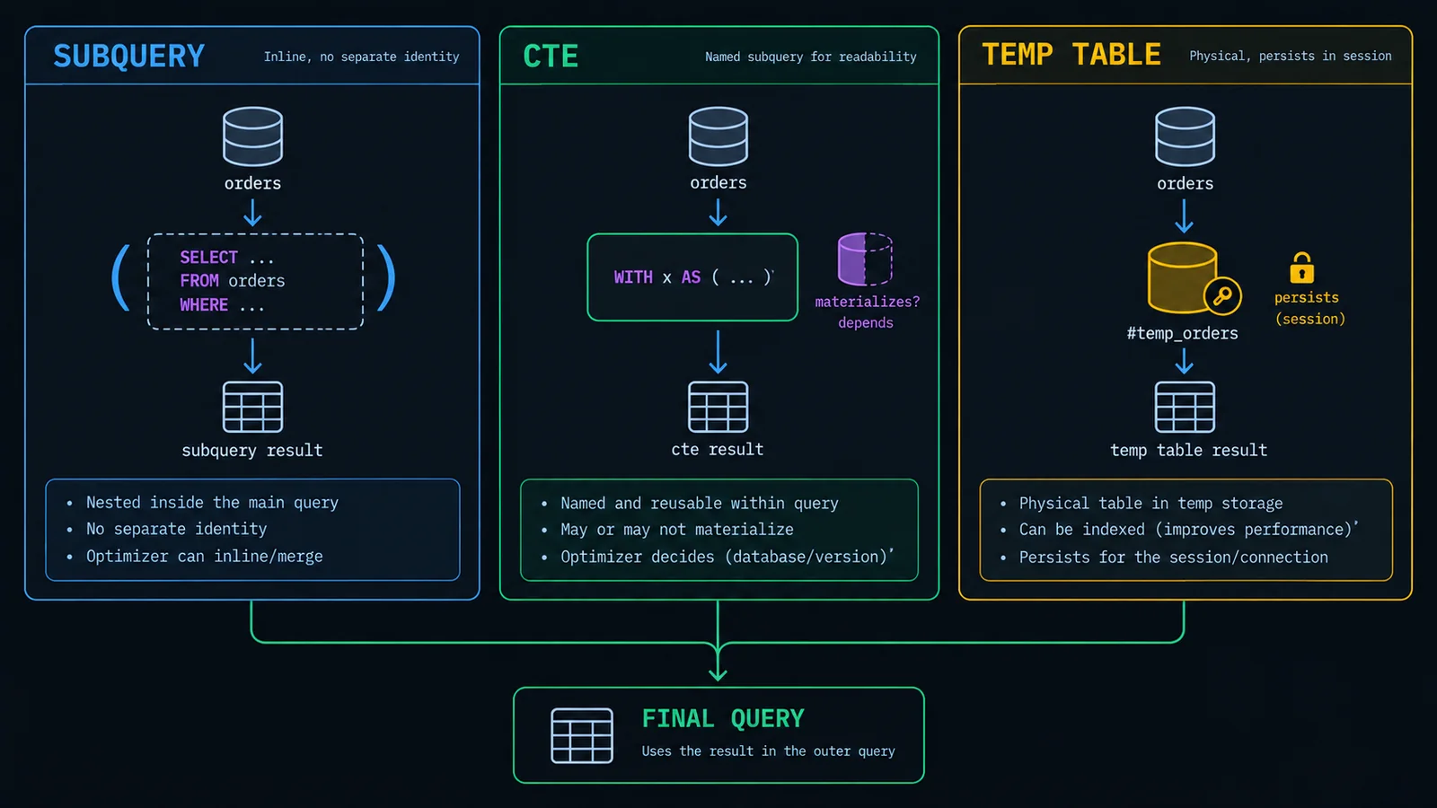
Every non-trivial query eventually needs to break a big problem into smaller, named pieces — compute a subtotal here, filter down a candidate set there, then combine those with something else downstream. SQL gives you three fundamentally different tools for that: a subquery nested inline, a CTE declared with WITH, or a temp table built as an explicit prior step. They can express identical logic and return identical rows, and for years the debate over which to use got settled with taste — "CTEs are more readable," "subqueries are for simple filters," "temp tables are only for huge datasets." Those rules aren't wrong so much as incomplete: each tool has a genuinely different cost profile depending on the engine you're running, and picking between them by feel is how a query that should take four seconds ends up taking seven minutes, with nobody quite sure why.
This piece works through all three in enough depth to make an informed choice rather than a habitual one: what a subquery is syntactically and how a correlated one executes differently from a non-correlated one, how CTEs read and chain, what recursive CTEs are for and how to write one without an infinite loop, when a real temp table earns its keep, and — the part that actually changes behavior in production — whether your specific engine treats a CTE as a readability aid it inlines away for free, or a hard boundary it can't optimize across. We'll close with a decision framework and the same multi-step query written all three ways, so the trade-offs are visible side by side instead of argued about in the abstract.
The Three Tools, and What They Have in Common
A subquery is a SELECT statement written inside another statement — inside a WHERE clause, inside the FROM clause as a derived table, inside the SELECT list as a scalar expression, or as the argument to IN, EXISTS, or a comparison operator. It has no name of its own unless you alias the derived table, no independent existence outside the statement that contains it, and the engine is free to fold it into the surrounding plan however it sees fit. You write it once, in place, and it disappears the moment the outer query finishes.
A CTE — a common table expression, declared with a leading WITH clause — is syntactically almost the same idea with a name attached up front. Instead of nesting a SELECT inline where you use it, you declare it once at the top of the statement, give it a name, and reference that name one or more times below. Nothing about the WITH clause guarantees anything about execution by itself; it's fundamentally a naming and sequencing construct. What actually happens underneath — whether the engine computes the CTE's result once and reuses it, or substitutes its definition everywhere it's referenced and recomputes it each time — depends entirely on the engine and, for at least one major engine, the exact version. That distinction is the single most consequential thing in this article, and it gets a full section of its own further down.
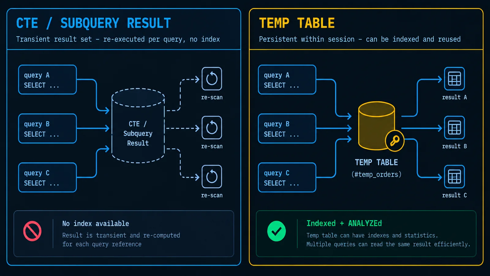
A temp table is a different kind of object entirely: an actual table, created with CREATE TEMPORARY TABLE, CREATE TABLE #name in SQL Server, or a session-scoped equivalent, populated by a separate INSERT INTO ... SELECT or CREATE TABLE ... AS SELECT, and queried afterward as its own object. It has real, computed-once rows sitting on disk or in memory, real statistics the optimizer can use, and — critically — it can carry its own indexes. It persists for the length of the session or transaction, which means you can query it more than once across multiple statements, not just multiple times inside one.
All three exist to solve the same underlying problem: a single SELECT, however cleverly structured, eventually becomes too dense to read, too repetitive to maintain, or too expensive to compute more than once. Breaking it into named pieces is good practice regardless of the mechanism — the question this article actually answers is what each mechanism costs once the query stops being trivial: what the optimizer can and can't see across the boundary, whether the intermediate result gets computed once or several times, whether you can index it, and how easy the whole thing is to debug when it returns the wrong row count during an incident.
| property | subquery | cte | temp table |
|---|---|---|---|
| Scope | single statement | single statement | session / transaction |
| Reusable across statements | no | no | yes |
| Independently indexable | no | no | yes |
| Guaranteed single computation | no | engine-dependent | yes |
| Own statistics for the optimizer | no | no (usually estimated) | yes, after ANALYZE / equivalent |
| Best for | a quick inline filter or existence check | readable, linear multi-step logic within one query | expensive, reused, or indexable intermediate results |
Subqueries Explained: Inline, Correlated vs. Non-Correlated
A subquery shows up in three shapes in practice. A scalar subquery returns exactly one row and one column and can be used anywhere a single value is expected — in a SELECT list, in a comparison like = (SELECT ...), in a default expression. A row or table subquery returns a set of rows and is used with IN, EXISTS, ANY, or ALL. And a derived table is a subquery used in place of a table name in the FROM clause, given an alias so its columns can be referenced — this shape is functionally almost identical to an unnamed, single-use CTE, and most modern optimizers treat the two the same way once parsing is done.
The distinction that actually matters for how a subquery executes is whether it's correlated or non-correlated. A non-correlated subquery is self-contained — it doesn't reference any column from the query that contains it, so it can, in principle, be evaluated entirely on its own before the outer query even starts.
SELECT customer_id, name
FROM customers
WHERE customer_id IN (
    SELECT customer_id
    FROM orders
    WHERE order_date >= '2026-05-01'
);
The inner query here doesn't need anything from customers — it can be computed once, producing a list of qualifying customer IDs, and the outer query just checks membership against that list. A correlated subquery, by contrast, references a column from the outer query inside its own WHERE clause, which means its result set genuinely depends on which outer row is currently being evaluated.
SELECT c.customer_id, c.name
FROM customers c
WHERE EXISTS (
    SELECT 1
    FROM orders o
    WHERE o.customer_id = c.customer_id
    AND o.order_date >= '2026-05-01'
);
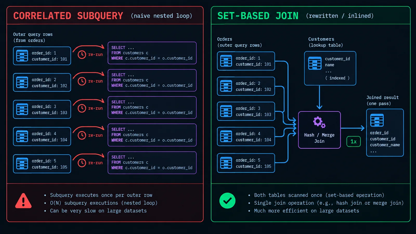
The naive mental model for a correlated subquery is a nested loop: for every row the outer query produces, plug that row's c.customer_id into the inner query and re-run it. That model is a reasonable first approximation and, for a subquery the optimizer can't rewrite, it's often close to literally what happens. But modern cost-based optimizers frequently transform well-formed correlated subqueries — especially ones wrapped in EXISTS or NOT EXISTS — into semi-joins or anti-joins internally, which execute as a single set-based join rather than a row-by-row loop. Whether that rewrite happens depends on the shape of the subquery, the engine, and sometimes the specific version; a subquery that references outer-query columns inside an aggregate, a window function, or a correlated ORDER BY/LIMIT is much less likely to be rewritable, and will tend to execute closer to the naive loop model. This is one of the reasons the join-vs-subquery framing matters as much as it does — our deep dive on SQL joins covers exactly how the engine decides between nested-loop, hash, and merge join strategies once a correlated pattern gets rewritten into one.
The EXISTS form above is worth contrasting with the equivalent written as IN and, separately, as a join — because the three aren't quite interchangeable once NULLs are involved. EXISTS only cares whether at least one matching row exists; it never has to inspect the actual values being compared beyond the join predicate, and it short-circuits on the first match. IN against a subquery has to build (or at least conceptually build) the full candidate list first. The dangerous case is NOT IN: if the subquery's result set contains even a single NULL, NOT IN silently returns zero rows for the entire outer query, because SQL's three-valued logic makes x NOT IN (1, 2, NULL) evaluate to unknown rather than true for every value of x, including values that clearly aren't 1 or 2. NOT EXISTS doesn't have this problem, because it never compares against the subquery's values directly — it just checks for the presence or absence of a matching row. If there's one habit worth building from this section alone, it's default to NOT EXISTS over NOT IN whenever the subquery's column can contain NULL, which in practice is most of the time.
The other place correlated subqueries quietly cost more than they look like they should is inside the SELECT list itself, computing one value per output row.
SELECT
    c.customer_id,
    c.name,
    (SELECT COUNT(*) FROM orders o WHERE o.customer_id = c.customer_id) AS order_count,
    (SELECT MAX(o.order_date) FROM orders o WHERE o.customer_id = c.customer_id) AS last_order
FROM customers c;
This runs two separate correlated subqueries per customer row — each one, in the worst case, scanning or index-probing orders independently. On a few thousand customers against a well-indexed orders.customer_id, you likely won't notice. On a few million, or against a column without a supporting index, this is the pattern that turns a report into a timeout. The set-based fix is almost always a single aggregation joined once, or — when the shape allows it — a window function computed in one pass over the data instead of one subquery execution per output row:
SELECT
    c.customer_id,
    c.name,
    COALESCE(o.order_count, 0) AS order_count,
    o.last_order
FROM customers c
LEFT JOIN (
    SELECT customer_id, COUNT(*) AS order_count, MAX(order_date) AS last_order
    FROM orders
    GROUP BY customer_id
) o ON o.customer_id = c.customer_id;
That derived table in the FROM clause is itself an unnamed, single-use subquery — and this is a useful thing to notice early: syntactically, a derived table and a single-reference CTE are close to the same construct wearing different clothes. Whether you write this as a subquery here or pull it into a named CTE above the main query is almost entirely a readability decision at this point, not a performance one, because a well-behaved optimizer inlines both the same way. That equivalence is exactly why the next section exists — CTEs read differently, but underneath, for the common case, they very often compile down to exactly this.
CTEs Explained: Syntax, Readability, Chaining Multiple CTEs
A CTE moves a subquery out of the place it's used and gives it a name declared up front, using a WITH clause that sits before the main statement. The basic form names one result set and references it once below:
WITH active_customers AS (
    SELECT customer_id, name
    FROM customers
    WHERE status = 'active'
)
SELECT *
FROM active_customers
WHERE name LIKE 'A%';
On its own, that buys you almost nothing over writing the same thing as a derived table — the value shows up once you have more than one intermediate step, because a WITH clause can declare several CTEs in sequence, each one allowed to reference any CTE declared before it (not after — SQL reads top to bottom, and a CTE can't forward-reference one that hasn't been defined yet, only WITH RECURSIVE breaks that rule, and only to reference itself).
WITH recent_orders AS (
    SELECT customer_id, order_id, order_total, order_date
    FROM orders
    WHERE order_date >= CURRENT_DATE - INTERVAL '90 days'
),
customer_totals AS (
    SELECT customer_id,
           SUM(order_total) AS revenue_90d,
           COUNT(*) AS order_count_90d
    FROM recent_orders
    GROUP BY customer_id
),
ranked AS (
    SELECT ct.*,
           RANK() OVER (ORDER BY revenue_90d DESC) AS revenue_rank
    FROM customer_totals ct
)
SELECT c.name, r.revenue_90d, r.order_count_90d, r.revenue_rank
FROM ranked r
JOIN customers c ON c.customer_id = r.customer_id
WHERE r.revenue_rank <= 10;
The readability win here is real and specific: each CTE gets a name that describes what it holds — recent_orders, customer_totals, ranked — so the final SELECT reads almost like prose, and someone opening this query cold can understand the shape of the logic without mentally unwinding three levels of nested parentheses. Compare that to the same logic written as nested subqueries, where the innermost filter is buried three levels deep and the outermost SELECT is separated from the filter it depends on by pages of indentation. CTEs turn a query that reads inside-out into one that reads top-to-bottom, in the same order you'd explain it out loud, and that alone is worth the syntax for anything beyond a two-step query.
It's worth being precise about what a CTE name buys you and what it doesn't. It is not a variable, and it doesn't create a temporary object outside the statement — every reference to ranked above is still, conceptually, "run this SELECT again," even though it only appears once in this example. The name is purely a textual and logical convenience within a single statement; it disappears the moment the statement finishes, exactly like a subquery does, and nothing about declaring it with WITH inherently changes execution cost. Whether the engine computes customer_totals once and hands the result to ranked, or re-derives it every time it's touched, is an execution detail the syntax doesn't promise you either way — which is precisely the subject of the materialization section further down, and the reason a plain "CTEs are more readable but not always faster" caveat undersells how differently that plays out engine to engine.
One more thing worth naming here because it sets up a mistake covered later: nothing stops you from chaining ten or fifteen CTEs in one statement, and the syntax doesn't get any harder to write as the chain grows — but the readability benefit that made CTEs attractive in the first place inverts past a certain length. A three- or four-step chain reads like a recipe. A twelve-step chain, where step nine depends on a filter buried in step three and step eleven silently duplicates a join that step six already did, reads like an undebuggable wall of text that nobody wants to touch. The tool doesn't stop you; good judgment about scope has to.
Recursive CTEs: Hierarchies, Org Charts, and Generating a Date Spine
Every CTE covered so far solves problems with a fixed, known number of steps — join this, aggregate that, rank the result. A different class of problem doesn't have a fixed depth: an employee reports to a manager, who reports to another manager, who reports to another, for an unknown number of levels depending on where in the org chart you start. A category can be nested inside a parent category, nested inside another parent, arbitrarily deep. You could write a chain of self-joins to handle three or four levels, but that approach breaks the moment the real data goes one level deeper than you hardcoded for. A recursive CTE is the tool built specifically for this shape: unknown depth, self-referential structure, walked one level at a time until there's nothing left to walk.
The syntax has three required parts. An anchor member — a plain SELECT that produces the starting rows. A recursive member — a SELECT that references the CTE's own name, joining it back to the base table to find "the next level." And a UNION ALL connecting them, which the engine re-runs against the most recently produced rows until the recursive member returns nothing at all, at which point the recursion terminates.
WITH RECURSIVE reporting_chain AS (
    -- anchor: the starting employee
    SELECT employee_id, name, manager_id, 1 AS depth
    FROM employees
    WHERE employee_id = 501

    UNION ALL

    -- recursive member: walk one level up each pass
    SELECT e.employee_id, e.name, e.manager_id, rc.depth + 1
    FROM employees e
    JOIN reporting_chain rc ON e.employee_id = rc.manager_id
)
SELECT * FROM reporting_chain ORDER BY depth;
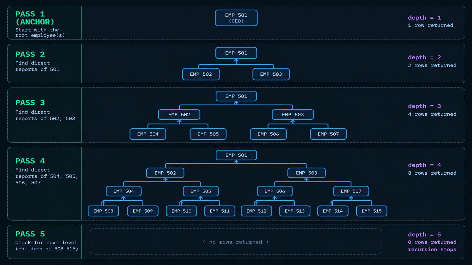
Trace it by hand once and the mechanics stop feeling like magic. Pass one runs the anchor and returns employee 501 at depth 1. Pass two runs the recursive member against only the rows produced by the previous pass — not the whole accumulated result — joining employees back to find whoever has manager_id matching 501's manager, producing depth 2. Pass three does the same thing against depth 2's row, and so on, until a pass produces zero rows because someone's manager_id is NULL — they're the CEO, nobody manages them, the recursive member finds nothing to join against, and the whole thing stops. The final result is every row produced across every pass, unioned together.
Two failure modes show up constantly with recursive CTEs, and both are worth knowing before you hit them in production rather than after. The first is a genuine infinite loop: if the underlying data has a cycle — an employee accidentally set as their own indirect manager through a data-entry error, a category that loops back to itself through a chain of parents — the recursive member never runs out of new rows to produce, and the query runs until something external stops it. Every engine has a safety valve for this, but the valves differ in shape. SQL Server enforces a MAXRECURSION limit of 100 by default and errors out past it (overridable per-query with OPTION (MAXRECURSION n), up to 32,767, or 0 for unlimited — use that last option carefully). MySQL, which added recursive CTE support in version 8.0, enforces a cte_max_recursion_depth session variable defaulting to 1,000 iterations. Postgres has no default iteration cap at all — a genuinely cyclic recursive CTE without explicit cycle protection will run until it exhausts memory or you kill it, which is the more dangerous default of the two philosophies. Postgres 14 added an explicit CYCLE clause for exactly this reason, letting you name the columns that define a cycle and have the engine detect and stop on one automatically rather than relying on depth limits as a blunt backstop.
WITH RECURSIVE reporting_chain AS (
    SELECT employee_id, name, manager_id
    FROM employees
    WHERE employee_id = 501

    UNION ALL

    SELECT e.employee_id, e.name, e.manager_id
    FROM employees e
    JOIN reporting_chain rc ON e.employee_id = rc.manager_id
)
CYCLE employee_id SET is_cycle USING path
SELECT * FROM reporting_chain;
The second failure mode is quieter: forgetting that UNION ALL, not UNION, is what you almost always want in the recursive term. UNION deduplicates on every pass, which for a genuinely tree-shaped hierarchy costs performance for no benefit, and for a cyclic graph can mask the cycle instead of surfacing it, since a row that would otherwise reappear (revealing the loop) gets silently collapsed away instead.
Recursive CTEs also solve a problem that has nothing to do with hierarchies on the surface: generating a sequence of values — most commonly, a date spine, one row per calendar day across a range, used to left-join real activity against so that days with zero orders or zero signups show up explicitly as zero rather than being silently absent from a report. Engines with a native sequence generator, like Postgres's generate_series, rarely need a recursive CTE for this. Engines without one — SQL Server has no built-in equivalent — lean on recursion instead:
WITH date_spine AS (
    SELECT CAST('2026-01-01' AS DATE) AS day_date
    UNION ALL
    SELECT DATEADD(DAY, 1, day_date)
    FROM date_spine
    WHERE day_date < '2026-12-31'
)
SELECT day_date FROM date_spine
OPTION (MAXRECURSION 400);
Note the explicit MAXRECURSION override — 365 days comfortably exceeds SQL Server's default cap of 100, and this is the single most common way people first meet that limit: not from a genuine bug, but from a perfectly correct date spine that's longer than the default assumes anyone would need. On engine support generally: Postgres, MySQL 8.0+, Snowflake, BigQuery (GoogleSQL), and Redshift all require the explicit RECURSIVE keyword — WITH RECURSIVE, not plain WITH — for a self-referencing CTE to parse at all. SQL Server is the outlier: it uses plain WITH for both recursive and non-recursive CTEs, with the recursive structure itself (a member referencing the CTE's own name) being what triggers recursive handling, no extra keyword required.
Temp Tables and Materialized Intermediate Tables
A temp table is the one option of the three that produces a real, physically computed object rather than a piece of query text the optimizer folds in somewhere. The syntax to create one varies by engine — Postgres and most Postgres-derived engines use CREATE TEMP TABLE or CREATE TEMPORARY TABLE, SQL Server uses a #-prefixed table name (session-scoped) or ## (globally visible across sessions, rarely what you want), Snowflake supports both true TEMPORARY tables scoped to the session and TRANSIENT tables with a longer but still limited lifecycle, and BigQuery — lacking persistent session state in the traditional sense — offers temp tables scoped to a multi-statement script rather than an open-ended session.
CREATE TEMP TABLE customer_totals AS
SELECT customer_id,
       SUM(order_total) AS revenue_90d,
       COUNT(*) AS order_count_90d
FROM orders
WHERE order_date >= CURRENT_DATE - INTERVAL '90 days'
GROUP BY customer_id;

CREATE INDEX ON customer_totals (customer_id);
ANALYZE customer_totals;

SELECT c.name, ct.revenue_90d
FROM customers c
JOIN customer_totals ct ON ct.customer_id = c.customer_id
WHERE ct.revenue_90d > 10000;
What that buys you over a CTE doing the identical aggregation is threefold, and each part matters for a different reason. First, the computation genuinely happens exactly once — there's no engine-specific ambiguity about whether it gets recomputed per reference, because it's a physical table you built with one explicit statement and query afterward as many times as you like, in the same statement or across several. Second, you can index it to match exactly how you're about to join or filter it, which a CTE's ephemeral result set never lets you do, no matter how the optimizer decides to handle it internally. Third, ANALYZE (or the equivalent statistics-collection step on your engine) gives the optimizer real, measured statistics about the temp table's actual row count and value distribution for every query that touches it afterward, rather than forcing the planner to estimate the cardinality of an intermediate result it's never materialized and has no history for — sight-unseen estimates are exactly where cardinality misestimation creeps in on deeply nested query plans, and a bad cardinality estimate early in a plan tends to compound into a badly chosen join order downstream.
None of that is free. Building a temp table means writing its rows out — to disk, to temp space, or at minimum into memory the engine has to manage — before you've gained anything from it, so for a small or cheap intermediate result, a temp table is pure overhead relative to a CTE or subquery the optimizer would have handled fine on its own. It's also an object with a lifecycle: it needs a name that doesn't collide with anything else in a reused session or connection pool, and depending on the engine and how you've scoped it, it may need explicit cleanup rather than just disappearing when the query finishes. In a connection-pooled application layer where sessions get reused across requests, a stray temp table from an earlier request that wasn't dropped is a real, if unglamorous, category of bug.
The trade-off here is close enough to the one dbt asks you to make explicitly at the model level, rather than inside a single query, that it's worth drawing the line directly: choosing between a CTE and a temp table inside one statement is functionally the same decision as choosing between an ephemeral model and a table (or incremental) materialization in dbt — do you want this intermediate step folded into the surrounding logic every time, or computed once and persisted as its own object with its own stats and indexes? Our guide to dbt materialization strategies walks through that same trade-off at the project level, and the reasoning transfers almost one for one.
Does a CTE Materialize or Inline? Engine by Engine
This is the question that actually determines whether "just use a CTE, it's more readable" is safe advice or a performance trap, and the honest answer is that it depends entirely on which engine you're running and, in Postgres's case, which version — so treat every claim below as something to verify against your own EXPLAIN output rather than take on faith, including from this article.
Postgres
Before Postgres 12 (released in October 2019), every CTE was always materialized, full stop — the community's shorthand for this was calling WITH an "optimization fence," because the planner could not push filters or conditions from the outer query down into the CTE's body, and could not push the CTE's output back out to be optimized jointly with the rest of the query. Whatever the CTE computed, it computed in full, wrote to a temporary internal buffer, and handed that fixed result to the rest of the query — reliable, but frequently slower than the equivalent subquery, because the planner lost the ability to reason across the boundary. Postgres 12 flipped the default: a non-recursive, side-effect-free CTE referenced exactly once is now inlined by default, folded into the query exactly as a subquery would be, with the planner free to push predicates in and optimize across the whole thing jointly. A CTE referenced more than once still defaults to the old materialize-once behavior, on the reasoning that materializing is usually the safer choice once something is computed and reused several times. You can override either default explicitly — AS MATERIALIZED forces the old fence behavior even for a single reference (useful when you deliberately want to stop the planner from pushing a filter into an expensive, function-heavy CTE it would otherwise re-run per outer row), and AS NOT MATERIALIZED forces inlining even for a CTE referenced multiple times, when you know duplication of that computation is cheaper than the alternative. Recursive CTEs and data-modifying CTEs (a CTE wrapping INSERT, UPDATE, or DELETE) are always materialized regardless of version, because inlining either one wouldn't be semantically safe.
WITH expensive_calc AS MATERIALIZED (
    SELECT customer_id, some_expensive_function(payload) AS score
    FROM raw_events
)
SELECT * FROM expensive_calc WHERE score > 90;
-- forces the calc to run once, even though it's referenced once here —
-- useful if you know a naive inline would let the planner push the
-- score > 90 filter in a way that re-runs the expensive function per row
-- under some plan shapes, when running it once up front is actually cheaper
Snowflake
Snowflake doesn't publish a hard, version-pegged default rule the way Postgres now does. Its cost-based optimizer treats a CTE largely as it treats a named subquery, deciding case by case whether to inline or to compute and reuse a result, based on how the CTE is used and referenced. A CTE referenced exactly once effectively never carries materialization overhead either way, since there's nothing to reuse. A CTE referenced multiple times is where the behavior is genuinely opportunistic rather than guaranteed — Snowflake's optimizer can recognize a repeated subexpression and compute it once, but that recognition isn't a documented contract you can rely on the way you can rely on an explicit temp table. If a CTE is doing real, expensive work and gets referenced more than once in the same statement, don't assume Snowflake will only pay for it once — check the query profile for the actual behavior on your specific query, and materialize explicitly to a temp table if the cost matters and you need certainty.
BigQuery
BigQuery's SQL dialect, GoogleSQL, is the most explicit of the four about this and takes the opposite default posture from modern Postgres: non-recursive CTEs are documented as not being materialized at all. If a non-recursive CTE is referenced N times in a query, GoogleSQL executes its definition N separate times — there is no shared computation, no automatic reuse, by design. A CTE that does a heavy join or aggregation and gets referenced three times in the surrounding query genuinely runs that join or aggregation three times. Recursive CTEs are the one exception and are materialized, because the recursive execution model requires it structurally — the engine has to hold the previous pass's result to feed into the next one. The practical upshot for BigQuery specifically: treat a repeatedly-referenced CTE as free readability sugar for logic used once, and reach for an actual staged table (a real table write, or a temp table scoped to a multi-statement script) the moment the same CTE gets referenced more than once and the underlying computation isn't cheap.
Redshift
Redshift's documentation describes an intent to optimize repeatedly-referenced WITH-clause subqueries as common subexpressions "where possible" — evaluating a CTE once and reusing the result across references — but in practice, and consistent with Redshift's Postgres-derived query planner heritage, a WITH clause commonly behaves as an optimization boundary similar to pre-12 Postgres: predicates from the surrounding query generally don't get pushed into the CTE body across that boundary. The honest summary is that Redshift's actual behavior is the least consistently documented of the four engines here, which is itself useful information — it means you should default to checking EXPLAIN for your specific query rather than assuming either inlining or reuse, and lean toward an explicit temp table (with a deliberately chosen distribution and sort key) whenever a CTE is doing meaningful work and feeds a large downstream join.
| engine | default for a non-recursive CTE | override |
|---|---|---|
| Postgres < 12 | always materialized (fence) | none available |
| Postgres 12+ | inlined if referenced once; materialized if referenced 2+ times | MATERIALIZED / NOT MATERIALIZED |
| Snowflake | cost-based, opportunistic — not a fixed rule | no explicit hint; verify via query profile |
| BigQuery (GoogleSQL) | always inlined / re-executed per reference (non-recursive) | none; use a staged table for reuse |
| Redshift | generally boundary-like; opportunistic reuse "where possible" | no explicit hint; verify via EXPLAIN |
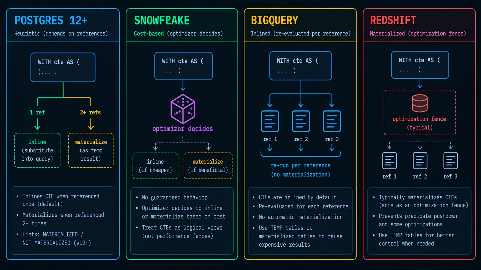
The pattern worth internalizing across all four isn't a specific rule so much as a posture: nothing about the WITH keyword itself is a performance promise on any engine. It's a readability and sequencing construct first, and whatever performance behavior rides along with it is a separate, engine-specific implementation detail that changes across versions and vendors. For a broader set of tactics beyond just this one decision — index selection, predicate pushdown, join order, and how to read an execution plan once you've picked your structure — see our companion piece on SQL and dbt query optimization techniques.
Indexing and Intermediate Results
Here's the distinction that follows directly from everything above, stated as plainly as possible: a temp table is a table, so it can have indexes built on exactly the columns your downstream query needs. A CTE or a subquery is not a table you have any handle on — even in the cases where an engine happens to materialize one internally, that materialized result is an anonymous, engine-managed intermediate spool, not an object you can run CREATE INDEX against. You get whatever access path the optimizer decides to build for that one query, built fresh, informed only by whatever estimate the planner has for that intermediate result's size and distribution.
This stops being an abstract distinction the moment an intermediate result needs to be joined against more than once, or joined on a column that isn't already the leading edge of an index on the base tables. Consider a CTE that aggregates a large orders table down to one row per customer, then gets joined against three separate downstream queries — one filtering on customer segment, one filtering on revenue tier, one joining to a marketing table on customer_id. Every one of those three queries, if the CTE isn't materialized by the engine, potentially re-triggers the full aggregation over the base orders table from scratch. Even where the engine does materialize it, that materialized result has no index of its own — every downstream lookup against it is a scan or, at best, whatever incidental ordering the aggregation happened to produce.
CREATE TEMP TABLE customer_agg AS
SELECT customer_id, segment, SUM(order_total) AS revenue
FROM orders o
JOIN customers c USING (customer_id)
GROUP BY customer_id, segment;

CREATE INDEX idx_customer_agg_segment ON customer_agg (segment);
CREATE INDEX idx_customer_agg_customer ON customer_agg (customer_id);
ANALYZE customer_agg;

-- three downstream queries now each get a real access path,
-- against real, measured statistics, instead of re-deriving the
-- aggregation or scanning an unindexed intermediate result three times
The statistics half of this matters as much as the index half and gets less attention. Once a temp table is populated, running ANALYZE (Postgres, Redshift) or the equivalent gives the optimizer a real row count and a real value-distribution histogram for that specific intermediate result — which lets it make an informed choice about join algorithm and join order for every query that touches it afterward. A CTE or subquery the planner hasn't materialized has no such history; its cardinality has to be estimated as part of one larger plan, propagated through however many joins and filters sit between the CTE's definition and wherever its output actually gets consumed. Estimation error compounds with each additional join in a plan — a CTE whose true row count is misjudged by 10x at the first join can produce a plan that's off by orders of magnitude three joins later, because each subsequent estimate builds on the one before it. This is one of the more common quiet causes of a deeply-chained CTE query that "used to be fast" degrading sharply after the underlying data grew, with no code change to point to — the plan the optimizer builds today, based on estimates rather than measurements, simply isn't the plan it built a year ago against a much smaller table.
A Decision Framework
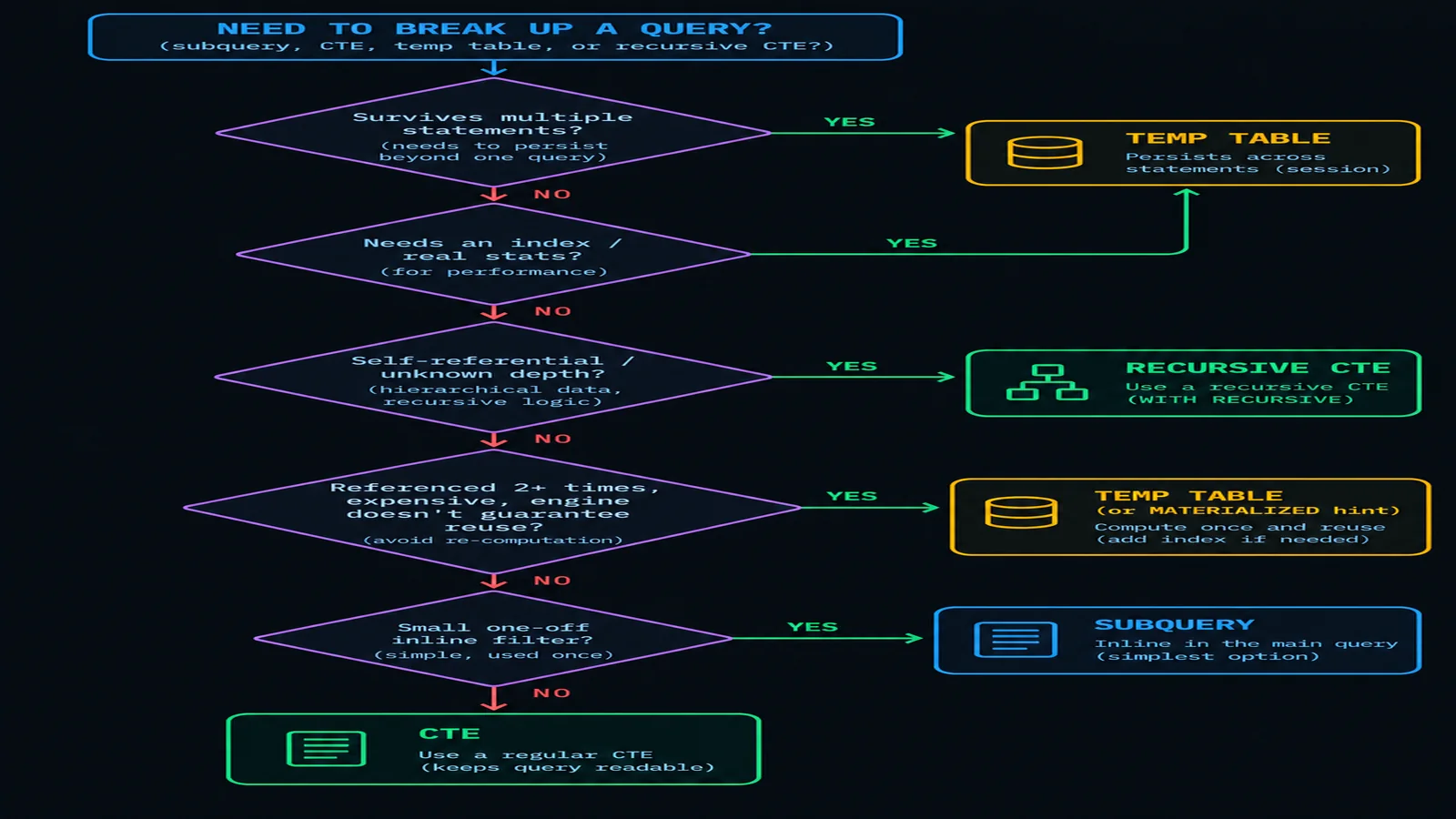
Rather than a flowchart with a single correct path, this is closer to a short sequence of questions, each one capable of settling the decision on its own before you need to ask the next.
Does the logic need to survive across more than one statement — a multi-step stored procedure, a script that stages rows and then runs several separate operations against them, a debugging session where you want to inspect an intermediate result interactively? If yes, a temp table is the only one of the three that can do this at all; neither a CTE nor a subquery has any existence outside the single statement that declares it, so this question alone settles the decision when it applies.
Does the intermediate result need an index, or does the downstream query need real statistics on it to get a good plan — because it's large, because it's joined more than once, or because it's joined on a column that isn't already well-indexed on the base tables? If yes, materialize it as a temp table, even within a single statement, and build the index to match how it's actually queried afterward.
Is the same expensive computation referenced more than once in one statement, on an engine that doesn't guarantee — or actively doesn't perform — shared computation for a repeated CTE reference? BigQuery, by documented default, and Snowflake and Redshift, without a firm guarantee either way, all fall into "verify before you trust it." If the computation is genuinely expensive and referenced multiple times, either force materialization where the engine supports an explicit hint (Postgres's MATERIALIZED), or fall back to a temp table, which sidesteps the question entirely by making single computation a structural fact rather than an optimizer decision.
Is the problem self-referential or of unknown depth — a hierarchy, a bill of materials, a graph walk? A recursive CTE is the only one of the three tools built to solve this without hardcoding a fixed number of self-joins that breaks the moment real data goes one level deeper.
Is this a small, single-use filter or existence check, nested exactly where it's needed, where naming it would add ceremony without adding clarity? A plain subquery, usually as EXISTS or IN, is the leanest tool and often the most honest representation of "this is a one-off condition, not a reusable concept."
Otherwise — multi-step, linear, readable-top-to-bottom logic within a single query, with no strong performance or persistence requirement pulling toward a temp table — a CTE is very often the right default, precisely because it's the option optimized for how the next person (including you, in six months) reads the query, not for anything about how the engine executes it.
Common Mistakes
Reusing an expensive correlated subquery in the SELECT list. Two or three correlated scalar subqueries in one row's output, each re-scanning or re-probing a large table per row, is a pattern that scales terribly and is almost always better expressed as a single aggregation joined once, or a window function computed in one pass. It's easy to write this way by instinct — it reads naturally, one subquery per computed column — and easy to miss how many times it's actually executing until the row count grows.
Chaining a dozen CTEs into an undebuggable pipeline. Nothing in the syntax caps how many CTEs you can declare in one WITH clause, but past four or five steps, the readability CTEs are supposed to buy you starts reversing — later steps depend on filters and joins buried several screens up, nobody can inspect step nine in isolation without copy-pasting it into a scratch query, and a bug three steps from the end can genuinely originate in step two. If a chain is growing past what fits comfortably on one screen, it's usually a sign that some of those steps deserve to be their own view, their own staged table, or split into a separate statement entirely.
Assuming a CTE referenced multiple times is computed once, on every engine, by default. That's true on Postgres 12+ (as the default, not a guarantee you should treat as permanent — it can still be overridden), unreliable on Snowflake and Redshift, and flatly false by design on BigQuery for non-recursive CTEs. Carrying a mental model from one engine into another without checking is exactly how "this ran fine in dev" turns into a production surprise the moment the same query runs against a different warehouse.
Using NOT IN against a subquery that can return NULL. If even one row in the subquery's result is NULL, the entire outer NOT IN silently evaluates to no rows matching, for every value being checked — not an error, not a warning, just a query that quietly returns nothing or far less than expected. NOT EXISTS doesn't have this failure mode and should be the default whenever the subquery's column isn't provably non-nullable.
Filtering on the "keep everything" side of an outer join wrapped around a CTE or subquery, inside WHERE instead of the join condition. This one isn't unique to CTEs, but it shows up constantly once logic gets wrapped in a named intermediate step — a filter that looks harmless in WHERE silently converts an outer join back into something that behaves like an inner join, because a comparison against NULL evaluates to unknown, and WHERE drops unknown rows. If you want to filter the joined side while still keeping unmatched rows from the preserved side, the condition belongs in the join's ON clause, not WHERE — this is covered in more depth, with worked examples, in our guide to SQL joins.
Reaching for a temp table by default, "just in case," for logic that would have been fine as a plain CTE. The opposite mistake gets less attention because it fails quietly rather than loudly — a temp table you didn't need still costs the write I/O to populate it, still needs a name that won't collide in a reused session, and still needs cleanup. If the intermediate result is small, computed once, and not reused across statements, a CTE is very often not just simpler to write but genuinely cheaper to run.
A Worked Comparison
To make the trade-offs concrete instead of abstract, here's one problem — "for each customer, their revenue and order count over the trailing 90 days, restricted to customers ranked in the top 10 by that revenue" — written all three ways against the same schema used earlier in this article.
SELECT c.name, ranked.revenue_90d, ranked.order_count_90d
FROM customers c
JOIN (
    SELECT customer_id, revenue_90d, order_count_90d,
           RANK() OVER (ORDER BY revenue_90d DESC) AS revenue_rank
    FROM (
        SELECT customer_id,
               SUM(order_total) AS revenue_90d,
               COUNT(*) AS order_count_90d
        FROM orders
        WHERE order_date >= CURRENT_DATE - INTERVAL '90 days'
        GROUP BY customer_id
    ) totals
) ranked ON ranked.customer_id = c.customer_id
WHERE ranked.revenue_rank <= 10;
Functionally correct, and on most modern optimizers this compiles to essentially the same plan as the CTE version below, since a derived table and a single-reference CTE are close to interchangeable once parsing is done. The cost is entirely readability: the innermost query — the actual aggregation, the part someone reading this query most wants to find first — is buried two levels of parentheses deep, and the ranking logic sits between the reader and it. Debugging this means either running the innermost SELECT in isolation by copy-pasting it out, or mentally tracking three levels of indentation at once.
WITH totals AS (
    SELECT customer_id,
           SUM(order_total) AS revenue_90d,
           COUNT(*) AS order_count_90d
    FROM orders
    WHERE order_date >= CURRENT_DATE - INTERVAL '90 days'
    GROUP BY customer_id
),
ranked AS (
    SELECT *, RANK() OVER (ORDER BY revenue_90d DESC) AS revenue_rank
    FROM totals
)
SELECT c.name, r.revenue_90d, r.order_count_90d
FROM ranked r
JOIN customers c ON c.customer_id = r.customer_id
WHERE r.revenue_rank <= 10;
Same logic, same likely execution plan on an engine that inlines single-reference CTEs — the difference is entirely that totals and ranked are named, so the final SELECT reads as "take the ranked totals, join customers, keep the top 10," in that order, matching how you'd say it out loud. If this needs to run on BigQuery and the CTEs stay single-reference as written here, there's no materialization penalty either way — this is the case where a CTE is close to a strictly-better rewrite of version A, readability with no engine-specific cost attached, though it's always worth confirming with your engine's plan rather than assuming.
CREATE TEMP TABLE customer_totals_90d AS
SELECT customer_id,
       SUM(order_total) AS revenue_90d,
       COUNT(*) AS order_count_90d
FROM orders
WHERE order_date >= CURRENT_DATE - INTERVAL '90 days'
GROUP BY customer_id;

CREATE INDEX ON customer_totals_90d (revenue_90d DESC);
ANALYZE customer_totals_90d;

SELECT c.name, ct.revenue_90d, ct.order_count_90d
FROM customer_totals_90d ct
JOIN customers c ON c.customer_id = ct.customer_id
ORDER BY ct.revenue_90d DESC
LIMIT 10;
For this specific query, run once, version C is very likely overkill — the extra write I/O to populate and index a temp table for a single downstream read buys nothing over version B. Where version C earns its cost is if customer_totals_90d gets reused: a dashboard that runs several different top-N and threshold queries against the same 90-day revenue base within one session, an ETL step that needs this exact aggregation available to more than one downstream transformation, or a case where the base orders aggregation is genuinely expensive and the engine in question (BigQuery, notably) won't share the computation across CTE references even within a single statement. Note also that version C swaps the window-function rank for a plain ORDER BY ... LIMIT 10 — with the aggregation already materialized and indexed on revenue_90d, there's no need to compute an explicit rank column at all if ties don't need to be reported, which is itself a small illustration of how materializing a step earlier can simplify what comes after it.
If you want to see these differences for yourself rather than take any of this on faith, the fastest path is running each version's EXPLAIN output through your own engine and comparing plan shapes directly — a tool like tools.techedge.in's SQL formatter is useful for getting all three versions into a consistent, comparable layout before you start reading plans side by side.
Wrapping Up
None of these three tools is the "right" one in any general sense — they're the right one for a specific set of constraints, and the constraints change the answer. A subquery is the leanest choice for a one-off, single-use condition, and adding a name to it via a CTE buys you nothing when it's only ever going to be read once, right where it's written. A CTE is the best default for multi-step logic that lives and dies within one query, precisely because it's optimized for how a person reads it rather than for any particular execution guarantee — a guarantee that, as the engine-by-engine section above should make clear, you can't assume transfers from one warehouse to another, or even across two major versions of the same one. A temp table earns its cost the moment an intermediate result needs to survive past one statement, needs its own index, or needs real statistics rather than an estimate buried three joins deep in a larger plan.
If there's one habit worth taking from this article beyond the specific rules, it's to stop treating "CTE vs. subquery vs. temp table" as a style preference and start treating it as a question with an actual, checkable answer for the query and engine in front of you. Run the EXPLAIN. Check whether your engine and version inline or materialize a CTE referenced more than once. Notice when a chain of CTEs has grown past what anyone could debug by reading it top to bottom. The syntax rarely stops you from making the wrong choice — only the plan does.
— Rakesh
EXPLAIN output before relying on any edge case in production.
One email, every other week.
New posts on data engineering, applied AI, and the business decisions around them. No noise, unsubscribe anytime.
Comments
All comments are reviewed before they appear publicly — this keeps spam out.
Loading comments…